|
|
|


|
1
|
|
2
|
In the Select Physics tree, select Electrochemistry > Electrodeposition, Deformed Geometry > Electrodeposition, Tertiary with Electroneutrality.
|
|
3
|
Click Add.
|
|
4
|
In the Concentrations (mol/m³) table, enter the following settings:
|
|
5
|
Click
|
|
6
|
In the Select Study tree, select Preset Studies for Selected Physics Interfaces > Time Dependent with Initialization.
|
|
7
|
Click
|
|
1
|
|
2
|
|
3
|
Click
|
|
4
|
Browse to the model’s Application Libraries folder and double-click the file cu_trench_deposition_parameters.txt.
|
|
1
|
|
2
|
|
3
|
|
4
|
|
5
|
|
6
|
|
1
|
|
2
|
|
3
|
|
4
|
|
5
|
|
6
|
Click
|
|
7
|
|
1
|
|
2
|
|
3
|
Clear the Keep interior boundaries checkbox.
|
|
4
|
Click in the Graphics window and then press Ctrl+A to select both objects.
|
|
1
|
|
2
|
|
3
|
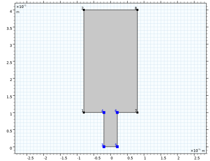
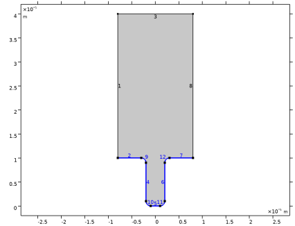
Select the Show geometry labels checkbox.
|
|
1
|
|
2
|
|
3
|
|
4
|
|
1
|
|
2
|
|
1
|
In the Model Builder window, under Component 1 (comp1) > Tertiary Current Distribution, Nernst–Planck (tcd) click Species Charges 1.
|
|
2
|
|
3
|
|
4
|
|
1
|
|
2
|
|
3
|
|
4
|
|
1
|
|
3
|
|
4
|
Click
|
|
5
|
|
6
|
Click OK.
|
|
7
|
In the Settings window for Electrode Surface, locate the Electrode Phase Potential Condition section.
|
|
8
|
|
9
|
|
1
|
|
2
|
|
3
|
|
4
|
In the Stoichiometric coefficients for dissolving–depositing species: table, enter the following settings:
|
|
5
|
|
6
|
|
1
|
In the Model Builder window, under Component 1 (comp1) > Tertiary Current Distribution, Nernst–Planck (tcd) right-click Electrode Surface 1 and choose Duplicate.
|
|
2
|
|
3
|
|
5
|
Click
|
|
6
|
|
7
|
Click OK.
|
|
8
|
In the Settings window for Electrode Surface, locate the Electrode Phase Potential Condition section.
|
|
9
|
|
1
|
|
2
|
|
3
|
In the Stoichiometric coefficients for dissolving–depositing species: table, enter the following settings:
|
|
1
|
In the Model Builder window, under Component 1 (comp1) > Tertiary Current Distribution, Nernst–Planck (tcd) click Initial Values 1.
|
|
2
|
|
3
|
|
1
|
|
2
|
|
3
|
|
4
|
|
1
|
In the Model Builder window, under Component 1 (comp1) right-click Mesh 1 and choose Edit Physics-Induced Sequence.
|
|
1
|
|
2
|
|
3
|
|
4
|
Click the Custom button.
|
|
5
|
|
6
|
|
7
|
|
8
|
Click
|
|
1
|
|
2
|
|
3
|
|
4
|
|
1
|
|
2
|
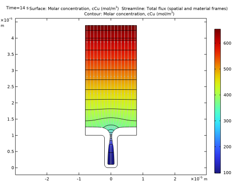
In the Settings window for Contour, click Replace Expression in the upper-right corner of the Expression section. From the menu, choose Component 1 (comp1) > Tertiary Current Distribution, Nernst–Planck > Species cCu > cCu - Molar concentration, cCu - mol/m³.
|
|
3
|
|
4
|
|
5
|
Clear the Color legend checkbox.
|
|
1
|
|
2
|
|
3
|
|
4
|
|
5
|
|
6
|
|
1
|
|
2
|
|
3
|
|
4
|
|
5
|
|
6
|
|
7
|
|
8
|
|
1
|
|
2
|
|
3
|
|
4
|
|
5
|
Locate the Plot Settings section.
|
|
6
|
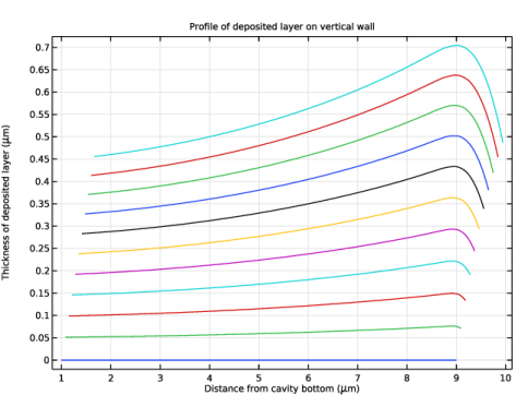
Select the x-axis label checkbox. In the associated text field, type Distance from cavity bottom (\mu m).
|
|
7
|
Select the y-axis label checkbox. In the associated text field, type Thickness of deposited layer (\mu m).
|
|
1
|
|
3
|
|
4
|
|
5
|
|
6
|
|
7
|
|
8
|
|
9
|
|
1
|
|
2
|
Go to the Add Study window.
|
|
3
|
Find the Studies subsection. In the Select Study tree, select Preset Studies for Selected Physics Interfaces > Time Dependent with Initialization.
|
|
4
|
Click the Add Study button in the window toolbar.
|
|
5
|
|
1
|
|
2
|
|
3
|
|
4
|
|
5
|
|
6
|
Clear the Generate default plots checkbox.
|
|
7
|
|
1
|
|
2
|
|
3
|
|
4
|
|
5
|
|
6
|
|
7
|