|
|
|
|
1
|
|
2
|
In the Select Physics tree, select Electrochemistry > Tertiary Current Distribution, Nernst–Planck > Tertiary, Electroneutrality (tcd).
|
|
3
|
Click Add.
|
|
4
|
|
5
|
In the Concentrations (mol/m³) table, enter the following settings:
|
|
6
|
In the Select Physics tree, select Fluid Flow > Multiphase Flow > Bubbly Flow > Bubbly Flow, Laminar Flow (bf).
|
|
7
|
Click Add.
|
|
8
|
Click
|
|
9
|
In the Select Study tree, select Preset Studies for Selected Physics Interfaces > Tertiary Current Distribution, Nernst–Planck > Time Dependent with Initialization.
|
|
10
|
Click
|
|
1
|
|
2
|
|
3
|
|
4
|
|
1
|
|
2
|
|
3
|
|
4
|
|
5
|
|
1
|
|
2
|
|
3
|
|
4
|
|
1
|
|
2
|
|
3
|
|
4
|
|
5
|
Click
|
|
1
|
|
2
|
|
3
|
Click
|
|
4
|
Browse to the model’s Application Libraries folder and double-click the file cu_electrowinning_bubbly_flow_parameters.txt.
|
|
1
|
In the Model Builder window, under Component 1 (comp1) click Tertiary Current Distribution, Nernst–Planck (tcd).
|
|
2
|
In the Settings window for Tertiary Current Distribution, Nernst–Planck, locate the Electrolyte Charge Conservation section.
|
|
3
|
|
1
|
In the Model Builder window, under Component 1 (comp1) > Tertiary Current Distribution, Nernst–Planck (tcd) click Species Charges 1.
|
|
2
|
|
3
|
|
4
|
|
5
|
|
1
|
|
2
|
|
3
|
|
4
|
|
5
|
|
6
|
|
7
|
|
8
|
|
1
|
|
2
|
|
4
|
Locate the Electrode Phase Potential Condition section. From the Electrode phase potential condition list, choose Total current.
|
|
5
|
|
1
|
In the Model Builder window, under Component 1 (comp1) > Tertiary Current Distribution, Nernst–Planck (tcd) > Anode Surface click Electrode Reaction 1.
|
|
2
|
In the Settings window for Electrode Reaction, type Oxygen Evolution Reaction in the Label text field.
|
|
3
|
|
4
|
|
5
|
|
6
|
|
1
|
|
3
|
|
4
|
|
1
|
In the Model Builder window, under Component 1 (comp1) > Tertiary Current Distribution, Nernst–Planck (tcd) > Cathode Surface click Electrode Reaction 1.
|
|
2
|
In the Settings window for Electrode Reaction, type Copper Deposition Reaction in the Label text field.
|
|
3
|
|
4
|
|
5
|
In the Stoichiometric coefficients for dissolving–depositing species: table, enter the following settings:
|
|
6
|
|
7
|
|
8
|
|
1
|
|
3
|
|
4
|
|
5
|
|
1
|
|
1
|
|
2
|
|
3
|
|
4
|
|
1
|
|
2
|
|
3
|
Clear the Low gas concentration checkbox.
|
|
1
|
In the Model Builder window, under Component 1 (comp1) > Bubbly Flow, Laminar Flow (bf) click Fluid Properties 1.
|
|
2
|
|
3
|
|
4
|
|
5
|
|
6
|
|
7
|
|
8
|
|
1
|
|
2
|
|
1
|
|
2
|
|
3
|
|
1
|
|
2
|
|
4
|
|
5
|
|
1
|
|
2
|
|
4
|
|
5
|
|
1
|
|
1
|
|
2
|
|
3
|
|
4
|
|
1
|
|
2
|
|
3
|
|
4
|
|
1
|
|
2
|
|
3
|
|
1
|
|
2
|
|
3
|
|
4
|
Click
|
|
1
|
|
2
|
|
3
|
|
5
|
|
6
|
|
7
|
Drag and drop below Size 1.
|
|
1
|
In the Model Builder window, expand the Boundary Layers 1 node, then click Boundary Layer Properties 1.
|
|
3
|
|
4
|
|
5
|
|
6
|
|
7
|
Click
|
|
1
|
In the Study toolbar, click
|
|
2
|
|
3
|
|
4
|
|
1
|
|
2
|
|
3
|
|
1
|
|
2
|
|
3
|
Right-click Study 1 > Solver Configurations > Solution 1 (sol1) > Time-Dependent Solver 1 and choose Fully Coupled.
|
|
4
|
|
1
|
|
2
|
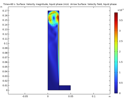
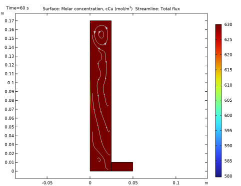
In the Settings window for Arrow Surface, click Replace Expression in the upper-right corner of the Expression section. From the menu, choose Component 1 (comp1) > Bubbly Flow, Laminar Flow > Velocity and pressure > u,v - Velocity field, liquid phase.
|
|
3
|
|
4
|
|
1
|
|
2
|
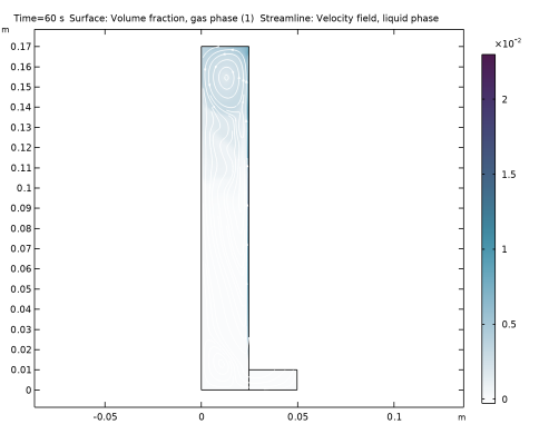
In the Settings window for Streamline, click Replace Expression in the upper-right corner of the Expression section. From the menu, choose Component 1 (comp1) > Bubbly Flow, Laminar Flow > Velocity and pressure > u,v - Velocity field, liquid phase.
|
|
3
|
|
4
|
|
5
|
Locate the Coloring and Style section. Find the Point style subsection. From the Type list, choose Arrow.
|
|
6
|
|
7
|
|
8
|
|
1
|
|
2
|
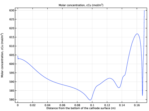
In the Settings window for 1D Plot Group, type Copper Concentration along Cathode Surface in the Label text field.
|
|
3
|
|
1
|
|
3
|
In the Settings window for Line Graph, click Replace Expression in the upper-right corner of the y-Axis Data section. From the menu, choose Component 1 (comp1) > Tertiary Current Distribution, Nernst–Planck > Species cCu > cCu - Molar concentration, cCu - mol/m³.
|
|
4
|
|
5
|
|
6
|
|
7
|
Select the Description checkbox. In the associated text field, type Distance from the bottom of the cathode surface.
|
|
8
|
|
1
|
|
2
|
|
3
|
|
4
|
|
1
|
|
2
|
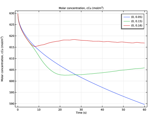
In the Settings window for 1D Plot Group, type Copper Concentration (Point Graph) in the Label text field.
|
|
1
|
|
2
|
|
3
|
|
4
|
Click Replace Expression in the upper-right corner of the y-Axis Data section. From the menu, choose Component 1 (comp1) > Tertiary Current Distribution, Nernst–Planck > Species cCu > cCu - Molar concentration, cCu - mol/m³.
|
|
5
|
|
6
|
|
1
|
|
2
|
|
3
|
|
4
|
|
5
|
|
1
|
|
2
|
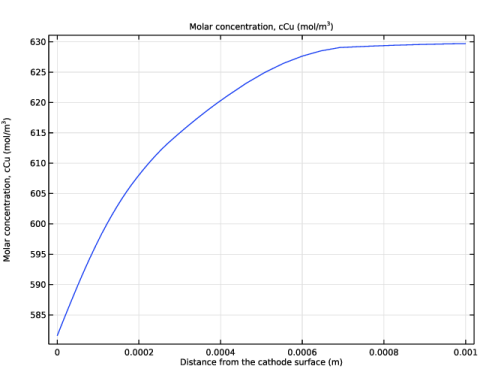
In the Settings window for 1D Plot Group, type Copper Concentration (Boundary Layer) in the Label text field.
|
|
1
|
|
2
|
|
3
|
|
4
|
|
5
|
Click Replace Expression in the upper-right corner of the y-Axis Data section. From the menu, choose Component 1 (comp1) > Tertiary Current Distribution, Nernst–Planck > Species cCu > cCu - Molar concentration, cCu - mol/m³.
|
|
6
|
|
7
|
|
8
|
Select the Description checkbox. In the associated text field, type Distance from the cathode surface.
|
|
9
|
|
1
|
|
2
|
|
3
|
|
1
|
|
3
|
|
4
|
Click to select the
|
|
6
|
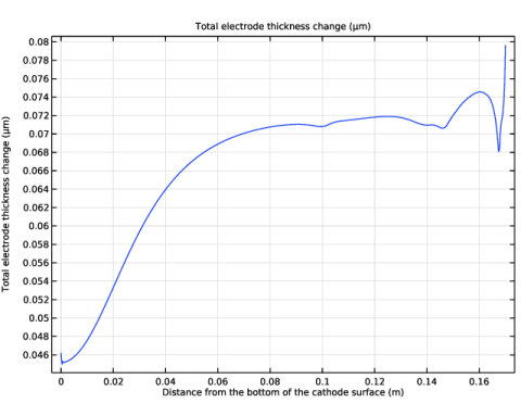
Click Replace Expression in the upper-right corner of the y-Axis Data section. From the menu, choose Component 1 (comp1) > Tertiary Current Distribution, Nernst–Planck > Dissolving–depositing species > tcd.sbtot - Total electrode thickness change - m.
|
|
7
|
|
8
|
|
9
|
|
10
|
Select the Description checkbox. In the associated text field, type Distance from the bottom of the cathode surface.
|
|
11
|