PDF

Alloy Deposition
Introduction
Electrochemical codeposition is a common low-cost method for producing metal alloys. This tutorial model demonstrates electrodeposition of a nickel (Ni)–phosphorous (P) alloy.
The model accounts for charge and mass transport of a multitude of species along with multiple electrode reactions such as Ni and P electrodeposition and hydrogen evolution. The model computes the steady state spatial distributions of the various species along the diffusion layer. The polarization plot along with deposition mole fraction plot reveal the desirable operating conditions for alloy preparation.
The model is based on a journal paper (Ref. 1).
Model Definition
The model is solved over a 1D computational domain that consists of a diffusion layer with an electrode surface at one end and a reference electrode at the other end, as shown in Figure 1. The electrolyte interval of length 0.02 cm is considered in the model.
Figure 1: Description of the model geometry including diffusion layer adjacent to the electrode surface.
Mass transport by convection, diffusion and migration for six species: H+, OH-, Ni2+, H3PO2, SO42-, and Na+, is solved using the Tertiary Current Distribution, Nernst-Planck interface:
where Ni denotes the transport vector (mol/(m2·s)), ci the concentration in the electrolyte (mol/m3), zi the charge for the ionic species, ui the mobility of the charged species (m2/(s·J·mole)), F Faraday’s constant (As/mole), and ϕl the potential in the electrolyte (V). The material balances are expressed through
where u denotes the velocity field.
The velocity in the normal direction to the electrode surface is defined by an analytical expression (originating from the von Karman and Cochran solution to the Navier-Stokes equations) as
where a ≈ 0.51 is a numerical parameter related to the velocity profile close to the surface, Ω is the rotation speed (rad/s), ν is the kinematic viscosity (m2/s), and x is the distance in the normal direction to the electrode surface (m).
All species along with their diffusion coefficients and reference concentrations are tabulated in Table 1.
D (m2/s)·109
cref (mol/m3)
Ni+2
H3PO2
SO4-2
H+
The concentration at the reference electrode boundary is set to the reference concentration for all species as tabulated in Table 1:
At the electrode surface boundary, an Electric potential boundary condition is used wherein the external electric potential, ϕs,ext, is set to the applied potential, which is varied from 0.5 V/SHE to 1.1 V/SHE in the interval of 0.025 V/SHE.
The water dissociation equilibrium reaction is built-in for the Tertiary Current Distribution, Nernst–Planck interface when using a water-based with electroneutrality charge conservation model:
Electrochemical reactions
The following electrochemical reactions occur at the electrode surface:
Nickel electrodeposition
Phosphorous electrodeposition
Hydrogen evolution
Butler-Volmer kinetics is used to model all electrochemical reactions, which will set the local current density according to
where i0,m is the exchange current density (A/m2), αa,m is the anodic transfer coefficient, αc,m is the cathodic transfer coefficient, F is the Faraday’s constant (96,485 C/mol), η,m is the overpotential (V), R is the Ideal gas constant (8.314 J/mol/K) and T is the temperature (K). The subscript m signifies the mth electrochemical reaction.
The η,m is calculated from
The equilibrium potentials for the electrochemical reactions are calculated using the Nernst equation accounting for its dependence on the ionic species concentration and relative activity of deposited species:
where is the standard electrode potential (V), nm is the number of electrons, ci,ref is the reference concentration of ionic species i (mol/m3), xj is the mole fraction of deposited species j, and aj,ref is the reference relative activity of deposited species j.
The exchange current density for the electrochemical reactions are described to account for its dependence on the ionic species concentration and relative activity of deposited species as,
where i0,ref,m is the reference exchange current density (A/m2).
At the electrode surface boundary, fluxes of ionic species are defined in terms of the electrochemical reactions as
where νi is the stoichiometric coefficient of ionic species i. This will set the flux to be proportional to the electrode current density according to Faraday’s law.
At the electrode surface boundary, the rate of deposition of deposited species is defined in terms of the electrochemical reactions as
where νd,j is the stoichiometric coefficient of deposited species j.
The mole fraction of deposited species is defined in terms of the rate of deposition as
Results and Discussion
Figure 2 shows the change in concentration for all species along the diffusion layer at applied potential of 0.8 V/SHE. It can be seen that the concentration gradient is the highest for Ni2+ at the electrode surface.
Figure 2: The change in concentration for all species along the diffusion layer at applied potential 0.8 V/SHE.
Figure 3 shows the polarization plot describing the change in cathodic (negative) total current density for different cathodic (negative) applied potentials at the electrode surface. The polarization plot shows larger cathodic current densities for larger cathodically applied potentials, with a plateau around -0.8 V/SHE.
Figure 3: The polarization plot showing the change in the cathodic (negative) current density for different cathodic (negative) applied potentials at the electrode surface.
Figure 4 shows the change in the deposition mole fraction for Ni and P for different cathodic (negative) applied potentials at the electrode surface. It can be seen that at potentials above the -0.8 V/SHE plateau, Ni is predominantly deposited at the electrode surface, whereas at potentials below the -0.8 V/SHE plateau, P starts getting deposited at the electrode surface, providing the desirable operating conditions for alloy deposition.
Figure 4: The change in deposition mole fraction for Ni and P for different cathodic (negative) applied potentials at the electrode surface.
Reference
1. S. Chen, K.-M. Yin, and R. E. White, “A Mathematical Model for the Electrodeposition of Alloys on a Rotating Disk Electrode,” J. Electrochem. Soc., vol. 135, no. 9, pp. 2193–2200, 1988.
Application Library path: Electrodeposition_Module/Tutorials/alloy_deposition
Modeling Instructions
From the File menu, choose New.
New
In the New window, click  Model Wizard.
Model Wizard
1
In the Model Wizard window, click  1D.
2
In the Select Physics tree, select Electrochemistry > Tertiary Current Distribution, Nernst–Planck > Tertiary, Water-Based with Electroneutrality (tcd).
3
Click Add.
4
In the Number of species text field, type 4.
5
In the Concentrations (mol/m³) table, enter the following settings:
6
Click  Study.
7
In the Select Study tree, select General Studies > Stationary.
8
Global Definitions
Load the model parameters from a text file.
Parameters 1
1
In the Model Builder window, under Global Definitions click Parameters 1.
2
In the Settings window for Parameters, locate the Parameters section.
3
Click  Load from File.
4
Geometry 1
The geometry consists of a linear segment describing the diffusion layer.
Interval 1 (i1)
1
In the Model Builder window, under Component 1 (comp1) right-click Geometry 1 and choose Interval.
2
In the Settings window for Interval, locate the Interval section.
3
4
Click  Build All Objects.
5
Click the  Zoom Extents button in the Graphics toolbar.
Definitions
Variables 1
Load the model variables from a text file.
1
In the Definitions toolbar, click  Local Variables.
2
In the Settings window for Variables, locate the Variables section.
3
Click  Load from File.
4
Tertiary Current Distribution, Nernst–Planck (tcd)
Start by defining the physics.
Species Charges 1
1
In the Model Builder window, under Component 1 (comp1) > Tertiary Current Distribution, Nernst–Planck (tcd) click Species Charges 1.
2
In the Settings window for Species Charges, locate the Charge section.
3
In the zcNi text field, type 2.
4
In the zcSO4 text field, type -2.
5
In the zcNa text field, type 1.
Electrolyte 1
1
In the Model Builder window, click Electrolyte 1.
2
In the Settings window for Electrolyte, locate the Convection section.
3
Specify the u vector as
4
Locate the Diffusion section. In the DcNi text field, type DNi.
5
In the DcH3PO2 text field, type DH3PO2.
6
In the DcSO4 text field, type DSO4.
7
In the DcNa text field, type DNa.
8
In the DcH text field, type DH.
9
In the DcOH text field, type DOH.
Initial Values 1
Set the initial values to the concentration of the species in the bulk.
1
In the Model Builder window, click Initial Values 1.
2
In the Settings window for Initial Values, locate the Initial Values section.
3
In the cNi text field, type cNi0.
4
In the cH3PO2 text field, type cH3PO20.
5
In the cSO4 text field, type cSO40.
6
In the cNa text field, type cNa0.
Electrode Surface 1
Set the electrode kinetics for multiple electrode reactions using the Electrode Surface node. Use the Dissolving-Depositing Species section to evaluate the rate of deposition for nickel and phosphorous at the electrode surface.
1
In the Physics toolbar, click  Boundaries and choose Electrode Surface.
2
3
In the Settings window for Electrode Surface, click to expand the Dissolving–Depositing Species section.
4
5
6
7
8
Locate the Electrode Phase Potential Condition section. In the ϕs,ext text field, type E_app.
Electrode Reaction: Ni Deposition
1
In the Model Builder window, under Component 1 (comp1) > Tertiary Current Distribution, Nernst–Planck (tcd) > Electrode Surface 1 click Electrode Reaction 1.
2
In the Settings window for Electrode Reaction, type Electrode Reaction: Ni Deposition in the Label text field.
3
Locate the Stoichiometric Coefficients section. In the n text field, type 2.
4
In the νcNi text field, type -1.
5
In the Stoichiometric coefficients for dissolving–depositing species: table, enter the following settings:
6
Locate the Equilibrium Potential section. In the Eeq,ref(T) text field, type Eeq_ref_Ni-R_const*T/(2*F_const)*log(max(xNi,eps^2)/aNi_ref).
7
Click to expand the Reference Concentrations section. In the table, enter the following settings:
8
Locate the Electrode Kinetics section. In the i0,ref(T) text field, type i0_ref_Ni*(max(xNi,eps)/aNi_ref)^0.75.
Electrode Surface 1
In the Model Builder window, click Electrode Surface 1.
Electrode Reaction: P Deposition
1
In the Physics toolbar, click  Attributes and choose Electrode Reaction.
2
In the Settings window for Electrode Reaction, type Electrode Reaction: P Deposition in the Label text field.
3
Locate the Stoichiometric Coefficients section. In the νcH3PO2 text field, type -1.
4
In the Stoichiometric coefficients for dissolving–depositing species: table, enter the following settings:
5
Locate the Equilibrium Potential section. In the Eeq,ref(T) text field, type Eeq_ref_P-R_const*T/(F_const)*log(max(xP,eps)/aP_ref).
6
Click to expand the Reference Concentrations section. In the table, enter the following settings:
7
In the cH,ref text field, type cH_ref.
8
Locate the Electrode Kinetics section. In the i0,ref(T) text field, type i0_ref_P*(max(xP,eps^2)/aP_ref)^0.5.
Electrode Surface 1
In the Model Builder window, click Electrode Surface 1.
Electrode Reaction: Hydrogen Evolution
1
In the Physics toolbar, click  Attributes and choose Electrode Reaction.
2
In the Settings window for Electrode Reaction, type Electrode Reaction: Hydrogen Evolution in the Label text field.
3
Locate the Equilibrium Potential section. In the Eeq,ref(T) text field, type Eeq_ref_H.
4
Click to expand the Reference Concentrations section. In the cH,ref text field, type cH_ref.
5
Locate the Electrode Kinetics section. In the i0,ref(T) text field, type i0_ref_H.
Concentration 1
Set concentrations of the species at the reference electrode boundary.
1
In the Physics toolbar, click  Boundaries and choose Concentration.
2
3
In the Settings window for Concentration, locate the Concentration section.
4
Select the Species cNi checkbox.
5
Select the Species cH3PO2 checkbox.
6
Select the Species cSO4 checkbox.
7
Select the Species cNa checkbox.
8
In the c0,cNi text field, type cNi0.
9
In the c0,cH3PO2 text field, type cH3PO20.
10
In the c0,cSO4 text field, type cSO40.
11
In the c0,cNa text field, type cNa0.
Electrolyte Potential 1
Set electrolyte potential at the reference electrode boundary to 0.
1
In the Physics toolbar, click  Boundaries and choose Electrolyte Potential.
2
Component 1 (comp1)
Now add a General Form Boundary PDE interface to solve for deposition mole fraction of Nickel.
Add Physics
1
In the Home toolbar, click  Add Physics to open the Add Physics window.
2
Go to the Add Physics window.
3
In the tree, select Mathematics > PDE Interfaces > Lower Dimensions > General Form Boundary PDE (gb).
4
Click to expand the Dependent Variables section. In the Dependent variables (1) table, enter the following settings:
5
Click the Add to Component 1 button in the window toolbar.
6
In the Home toolbar, click  Add Physics to close the Add Physics window.
General Form Boundary PDE (gb)
1
In the Settings window for General Form Boundary PDE, locate the Boundary Selection section.
2
3
Click  Remove from Selection.
4
5
Locate the Units section. In the Source term quantity table, enter the following settings:
General Form PDE 1
1
In the Model Builder window, under Component 1 (comp1) > General Form Boundary PDE (gb) click General Form PDE 1.
2
In the Settings window for General Form PDE, locate the Source Term section.
3
In the f text field, type xNi-xNi_expr.
4
Locate the Damping or Mass Coefficient section. In the da text field, type 0.
Initial Values 1
1
In the Model Builder window, click Initial Values 1.
2
In the Settings window for Initial Values, locate the Initial Values section.
3
In the xNi text field, type 1.
Global Definitions
Default Model Inputs
Set the default model input temperature to T.
1
In the Model Builder window, under Global Definitions click Default Model Inputs.
2
In the Settings window for Default Model Inputs, locate the Browse Model Inputs section.
3
In the tree, select General > Temperature (K) - minput.T.
4
Find the Expression for remaining selection subsection. In the Temperature text field, type T.
Mesh 1
Build a mesh using a finer resolution at the electrode surface.
1
In the Model Builder window, under Component 1 (comp1) click Mesh 1.
2
In the Settings window for Mesh, locate the Sequence Type section.
3
From the list, choose User-controlled mesh.
Size
1
In the Model Builder window, under Component 1 (comp1) > Mesh 1 click Size.
2
In the Settings window for Size, locate the Element Size section.
3
From the Predefined list, choose Extra fine.
Size 1
1
In the Model Builder window, click Size 1.
2
In the Settings window for Size, locate the Element Size section.
3
Click the Custom button.
4
Locate the Element Size Parameters section.
5
Select the Maximum element size checkbox. In the associated text field, type 1.0E-6.
Edge 1
In the Model Builder window, right-click Edge 1 and choose Build All.
Study 1
Step 1: Stationary
1
In the Model Builder window, under Study 1 click Step 1: Stationary.
2
In the Settings window for Stationary, click to expand the Study Extensions section.
3
Select the Auxiliary sweep checkbox.
4
5
6
In the Study toolbar, click  Compute.
Results
Several plots are added by default. The following steps reproduce the plots from the Results and Discussion section:
Concentrations, All Species (tcd)
1
In the Model Builder window, under Results click Concentrations, All Species (tcd).
2
In the Settings window for 1D Plot Group, locate the Data section.
3
From the Parameter selection (E_app) list, choose From list.
4
In the Parameter values (E_app (V)) list box, select -0.8.
5
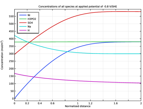
Click to expand the Title section. In the Title text area, type Concentrations of all species at applied potential of -0.8 V/SHE.
6
Locate the Plot Settings section.
7
Select the x-axis label checkbox. In the associated text field, type Normalized distance.
8
Select the y-axis label checkbox.
9
Locate the Axis section. Select the Manual axis limits checkbox.
10
In the x minimum text field, type 0.
11
In the x maximum text field, type 2.
12
Locate the Legend section. From the Position list, choose Upper left.
Species Ni
1
In the Model Builder window, expand the Concentrations, All Species (tcd) node, then click Species Ni.
2
In the Settings window for Line Graph, locate the x-Axis Data section.
3
In the Expression text field, type x/1.1517e-3[cm].
4
Click to expand the Coloring and Style section. From the Width list, choose 2.
Species H3PO2
1
In the Model Builder window, click Species H3PO2.
2
In the Settings window for Line Graph, locate the x-Axis Data section.
3
In the Expression text field, type x/1.1517e-3[cm].
4
Locate the Coloring and Style section. From the Width list, choose 2.
Species SO4
1
In the Model Builder window, click Species SO4.
2
In the Settings window for Line Graph, locate the x-Axis Data section.
3
In the Expression text field, type x/1.1517e-3[cm].
4
Locate the Coloring and Style section. From the Width list, choose 2.
Species Na
1
In the Model Builder window, click Species Na.
2
In the Settings window for Line Graph, locate the x-Axis Data section.
3
In the Expression text field, type x/1.1517e-3[cm].
4
Locate the Coloring and Style section. From the Width list, choose 2.
Species H
1
In the Model Builder window, right-click Species Na and choose Duplicate.
2
In the Settings window for Line Graph, type Species H in the Label text field.
3
Locate the y-Axis Data section. In the Expression text field, type tcd.cH.
4
Click to expand the Legends section. Find the Prefix and suffix subsection. In the Prefix text field, type H.
5
In the Concentrations, All Species (tcd) toolbar, click  Plot.
The plot should look like Figure 2.
Polarization Plot
Next, plot the polarization plot.
1
In the Results toolbar, click  1D Plot Group.
2
In the Settings window for 1D Plot Group, type Polarization Plot in the Label text field.
3
Locate the Title section. From the Title type list, choose Manual.
4
In the Title text area, type Polarization plot.
Point Graph 1
1
In the Polarization Plot toolbar, click  Point Graph.
2
3
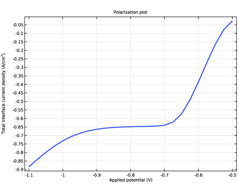
In the Settings window for Point Graph, click Replace Expression in the upper-right corner of the y-Axis Data section. From the menu, choose Component 1 (comp1) > Tertiary Current Distribution, Nernst–Planck > Electrode kinetics > tcd.itot - Total interface current density - A/m².
4
Locate the y-Axis Data section. In the Unit field, type A/cm^2.
5
Locate the x-Axis Data section. From the Parameter list, choose Expression.
6
In the Expression text field, type E_app.
7
Click to expand the Coloring and Style section. From the Width list, choose 2.
8
In the Polarization Plot toolbar, click  Plot.
The plot should look like Figure 3.
Deposition Mole Fraction
Finally, plot deposition mole fraction against the applied potential.
1
In the Results toolbar, click  1D Plot Group.
2
In the Settings window for 1D Plot Group, type Deposition Mole Fraction in the Label text field.
3
Locate the Title section. From the Title type list, choose Manual.
4
In the Title text area, type Deposition mole fraction.
5
Locate the Plot Settings section.
6
Select the x-axis label checkbox. In the associated text field, type Applied potential (V).
7
Select the y-axis label checkbox. In the associated text field, type Deposition mole fraction (1).
8
Locate the Legend section. From the Position list, choose Middle left.
Point Graph 1
1
In the Deposition Mole Fraction toolbar, click  Point Graph.
2
3
In the Settings window for Point Graph, locate the y-Axis Data section.
4
In the Expression text field, type xNi.
5
Locate the x-Axis Data section. From the Parameter list, choose Expression.
6
In the Expression text field, type E_app.
7
Locate the Coloring and Style section. From the Width list, choose 2.
8
Click to expand the Legends section. Select the Show legends checkbox.
9
From the Legends list, choose Manual.
10
Point Graph 2
1
Right-click Point Graph 1 and choose Duplicate.
2
In the Settings window for Point Graph, locate the y-Axis Data section.
3
In the Expression text field, type xP.
4
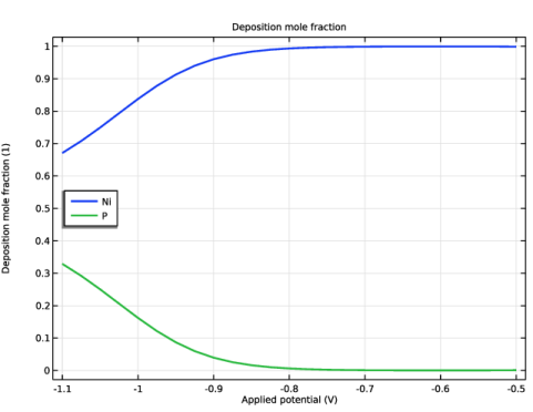
Locate the Legends section. In the table, enter the following settings:
5
In the Deposition Mole Fraction toolbar, click  Plot.
The plot should look like Figure 4.