|
|
|


|
1
|
|
2
|
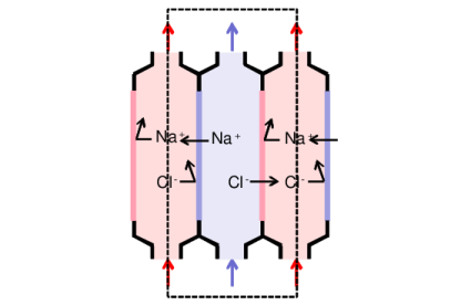
In the Select Physics tree, select Electrochemistry > Tertiary Current Distribution, Nernst–Planck > Tertiary, Electroneutrality (tcd).
|
|
3
|
Click Add.
|
|
4
|
In the Concentrations (mol/m³) table, enter the following settings:
|
|
5
|
Click
|
|
6
|
|
7
|
Click
|
|
1
|
|
2
|
|
3
|
Click
|
|
4
|
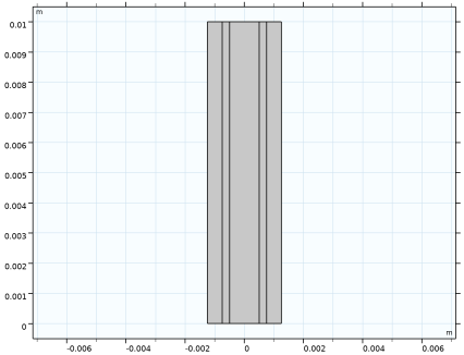
Browse to the model’s Application Libraries folder and double-click the file electrodialysis_parameters.txt.
|
|
1
|
|
2
|
|
3
|
|
4
|
|
5
|
|
6
|
Click
|
|
1
|
|
2
|
|
3
|
|
4
|
|
5
|
|
6
|
Click
|
|
1
|
|
2
|
|
3
|
|
4
|
|
5
|
|
6
|
Click
|
|
7
|
|
1
|
|
2
|
|
1
|
|
2
|
|
1
|
|
2
|
|
1
|
|
2
|
|
3
|
|
1
|
|
2
|
|
3
|
|
1
|
|
2
|
|
3
|
|
4
|
|
5
|
Locate the Units section. In the table, enter the following settings:
|
|
6
|
|
7
|
Locate the Plot Parameters section. In the table, enter the following settings:
|
|
1
|
|
2
|
|
3
|
|
5
|
Locate the Variables section. In the table, enter the following settings:
|
|
1
|
|
2
|
|
3
|
|
5
|
Locate the Variables section. In the table, enter the following settings:
|
|
1
|
|
2
|
|
3
|
|
5
|
Locate the Variables section. In the table, enter the following settings:
|
|
1
|
In the Model Builder window, under Component 1 (comp1) > Tertiary Current Distribution, Nernst–Planck (tcd) click Species Charges 1.
|
|
2
|
|
3
|
|
4
|
|
1
|
|
2
|
|
3
|
Specify the u vector as
|
|
4
|
|
5
|
|
1
|
|
2
|
In the Settings window for Ion-Exchange Membrane, type Ion-Exchange Membrane (Cation Selective) in the Label text field.
|
|
3
|
|
4
|
|
5
|
|
6
|
|
7
|
|
1
|
|
2
|
In the Settings window for Ion-Exchange Membrane, type Ion-Exchange Membrane (Anion Selective) in the Label text field.
|
|
3
|
|
4
|
|
1
|
|
3
|
|
4
|
|
5
|
Clear the Apply for electrode phase checkbox.
|
|
1
|
|
1
|
|
2
|
|
3
|
|
4
|
|
5
|
|
1
|
|
2
|
|
3
|
|
1
|
|
2
|
|
3
|
|
4
|
|
1
|
|
2
|
|
3
|
|
4
|
|
1
|
|
3
|
|
4
|
|
1
|
|
2
|
|
3
|
Click
|
|
5
|
|
6
|
|
7
|
|
8
|
Select the Symmetric distribution checkbox.
|
|
1
|
|
2
|
|
3
|
Click
|
|
5
|
|
6
|
Clear the Symmetric distribution checkbox.
|
|
7
|
Select the Reverse direction checkbox.
|
|
1
|
|
2
|
|
3
|
Click
|
|
5
|
|
1
|
|
2
|
|
3
|
Click
|
|
5
|
|
6
|
Select the Symmetric distribution checkbox.
|
|
7
|
|
1
|
|
2
|
|
3
|
|
4
|
|
5
|
|
1
|
|
2
|
|
3
|
|
4
|
|
1
|
|
2
|
|
3
|
|
4
|
|
5
|
|
6
|
|
1
|
|
2
|
|
3
|
|
4
|
|
1
|
|
2
|
|
3
|
|
4
|
|
5
|
Click
|
|
1
|
|
2
|
|
3
|
|
4
|
|
5
|
Locate the Plot Settings section.
|
|
6
|
|
1
|
|
2
|
|
1
|
|
2
|
|
3
|
|
4
|
|
5
|
Locate the Plot Settings section.
|
|
6
|
|
7
|
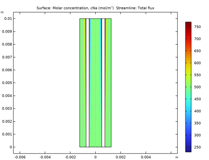
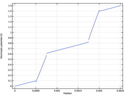
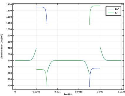
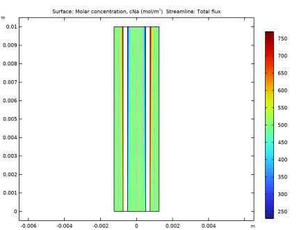
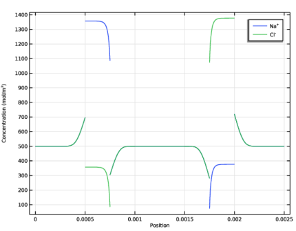
Select the y-axis label checkbox. In the associated text field, type Concentration (mol/m<sup>3</sup>).
|
|
1
|
|
2
|
|
3
|
|
4
|
|
5
|
|
1
|
|
2
|
|
3
|
|
4
|
|
5
|
|
7
|
|
1
|
|
2
|
|
3
|
|
1
|
|
2
|
|
3
|
|
4
|
|
5
|
|
1
|
|
2
|
|
3
|
|
4
|
Locate the Legends section. In the table, enter the following settings:
|
|
1
|
|
2
|
|
3
|
|
4
|
Locate the Legends section. In the table, enter the following settings:
|
|
1
|
|
2
|
|
3
|
|
4
|
|
5
|
|
6
|
|
7
|
|
1
|
|
2
|
|
1
|
|
2
|
|
3
|
|
1
|
|
2
|
|
3
|
|
1
|
|
2
|
|
3
|
|
4
|
|
1
|
|
2
|
|
1
|
|
2
|
|
3
|
Click to select the
|
|
5
|
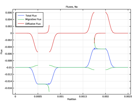
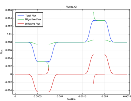
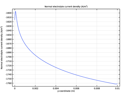
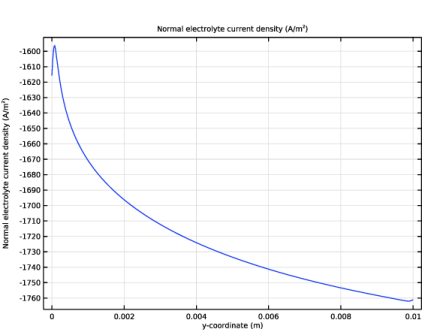
Click Replace Expression in the upper-right corner of the y-Axis Data section. From the menu, choose Component 1 (comp1) > Tertiary Current Distribution, Nernst–Planck > tcd.nIl - Normal electrolyte current density - A/m².
|
|
6
|
|
7
|
|
8
|