|
|
|


|
1
|
|
2
|
In the Select Physics tree, select Electrochemistry > Tertiary Current Distribution, Nernst–Planck > Tertiary, Electroneutrality (tcd).
|
|
3
|
Click Add.
|
|
4
|
In the Concentrations (mol/m³) table, enter the following settings:
|
|
5
|
In the Select Physics tree, select Fluid Flow > Porous Media and Subsurface Flow > Brinkman Equations (br).
|
|
6
|
Click Add.
|
|
7
|
In the Select Physics tree, select Mathematics > ODE and DAE Interfaces > Domain ODEs and DAEs (dode).
|
|
8
|
Click Add.
|
|
9
|
|
10
|
In the Dependent variables (1) table, enter the following settings:
|
|
11
|
Click
|
|
12
|
In the Dependent variable quantity table, enter the following settings:
|
|
13
|
In the Source term quantity table, enter the following settings:
|
|
14
|
In the Select Physics tree, select Mathematics > ODE and DAE Interfaces > Domain ODEs and DAEs (dode).
|
|
15
|
Click Add.
|
|
16
|
In the Source term quantity table, enter the following settings:
|
|
17
|
|
18
|
In the Dependent variables (1) table, enter the following settings:
|
|
19
|
Click
|
|
20
|
|
21
|
Click
|
|
1
|
|
2
|
|
3
|
|
4
|
Browse to the model’s Application Libraries folder and double-click the file capacitive_deionization_geometry.txt.
|
|
1
|
|
2
|
|
3
|
|
4
|
Browse to the model’s Application Libraries folder and double-click the file capacitive_deionization_electrolyte.txt.
|
|
1
|
|
2
|
|
3
|
|
4
|
Browse to the model’s Application Libraries folder and double-click the file capacitive_deionization_porous_electrode.txt.
|
|
1
|
|
2
|
In the Settings window for Parameters, type Porous Electrode, Attractive Potential in the Label text field.
|
|
3
|
|
4
|
Browse to the model’s Application Libraries folder and double-click the file capacitive_deionization_porous_electrode_attractive_potential.txt.
|
|
1
|
|
2
|
|
3
|
|
4
|
Browse to the model’s Application Libraries folder and double-click the file capacitive_deionization_flow.txt.
|
|
1
|
|
2
|
|
3
|
|
4
|
Browse to the model’s Application Libraries folder and double-click the file capacitive_deionization_process.txt.
|
|
1
|
|
2
|
|
3
|
|
4
|
Browse to the model’s Application Libraries folder and double-click the file capacitive_deionization_mesh.txt.
|
|
1
|
|
2
|
In the Settings window for Variables, type Donnan Condition and Current Balance in the Label text field.
|
|
3
|
|
4
|
Browse to the model’s Application Libraries folder and double-click the file capacitive_deionization_donnan_condition_current_balance.txt.
|
|
1
|
|
2
|
|
3
|
Locate the Variables section. In the table, enter the following settings:
|
|
1
|
|
2
|
In the Settings window for Variables, type Porous Electrode, Attractive Potential in the Label text field.
|
|
3
|
Locate the Variables section. In the table, enter the following settings:
|
|
1
|
|
2
|
In the Settings window for Variables, type Porous Electrode, Stern Layer Properties in the Label text field.
|
|
3
|
Locate the Variables section. In the table, enter the following settings:
|
|
1
|
|
2
|
|
3
|
Locate the Variables section. In the table, enter the following settings:
|
|
1
|
|
2
|
|
1
|
|
2
|
|
1
|
|
2
|
|
1
|
|
2
|
|
1
|
|
2
|
|
3
|
|
1
|
In the Model Builder window, expand the Component 1 (comp1) > Definitions > View 1 node, then click Axis.
|
|
2
|
|
3
|
|
4
|
|
1
|
|
2
|
|
3
|
|
4
|
|
1
|
|
2
|
|
3
|
|
4
|
|
5
|
|
1
|
|
2
|
|
3
|
|
4
|
|
5
|
|
1
|
|
2
|
|
3
|
|
4
|
|
5
|
|
6
|
|
1
|
|
2
|
|
3
|
|
4
|
|
5
|
|
6
|
|
1
|
|
2
|
|
3
|
|
4
|
|
5
|
Click OK.
|
|
6
|
|
7
|
|
1
|
In the Model Builder window, under Component 1 (comp1) > Definitions click Integration 1 (intop_upper_electrode).
|
|
1
|
|
1
|
|
1
|
|
1
|
|
2
|
|
3
|
|
1
|
|
2
|
Go to the Add Material window.
|
|
3
|
|
4
|
Click the Add to Component button in the window toolbar.
|
|
5
|
|
1
|
In the Model Builder window, under Component 1 (comp1) click Tertiary Current Distribution, Nernst–Planck (tcd).
|
|
2
|
In the Settings window for Tertiary Current Distribution, Nernst–Planck, locate the Out-of-Plane Thickness section.
|
|
3
|
|
1
|
In the Model Builder window, under Component 1 (comp1) > Tertiary Current Distribution, Nernst–Planck (tcd) click Species Charges 1.
|
|
2
|
|
3
|
|
4
|
|
1
|
|
2
|
|
3
|
|
4
|
|
5
|
|
1
|
|
2
|
|
3
|
|
1
|
|
3
|
|
4
|
|
5
|
|
6
|
|
7
|
|
8
|
|
9
|
|
1
|
|
1
|
|
3
|
|
4
|
|
1
|
|
1
|
|
1
|
|
3
|
|
4
|
From the list, choose Potentiostatic.
|
|
5
|
|
1
|
|
2
|
|
3
|
Select the Elapsed time checkbox.
|
|
4
|
|
1
|
|
2
|
|
3
|
|
4
|
|
1
|
|
3
|
|
4
|
|
5
|
|
6
|
|
1
|
In the Model Builder window, under Component 1 (comp1) > Brinkman Equations (br) > Porous Medium 1 click Porous Matrix 1.
|
|
2
|
|
3
|
|
4
|
|
1
|
In the Model Builder window, under Component 1 (comp1) > Brinkman Equations (br) click Initial Values 1.
|
|
2
|
|
3
|
Specify the u vector as
|
|
1
|
|
1
|
|
3
|
|
4
|
From the list, choose Fully developed flow.
|
|
5
|
|
1
|
|
3
|
|
4
|
Select the Normal flow checkbox.
|
|
1
|
|
2
|
In the Settings window for Domain ODEs and DAEs, type Domain ODEs and DAEs: Micropore Electrolyte Potential in the Label text field.
|
|
4
|
Click to expand the Dependent Variables section.
|
|
1
|
In the Model Builder window, under Component 1 (comp1) > Domain ODEs and DAEs: Micropore Electrolyte Potential (dode) click Distributed ODE 1.
|
|
2
|
|
3
|
|
4
|
|
1
|
|
2
|
In the Settings window for Domain ODEs and DAEs, type Domain ODEs and DAEs: Attractive Potential in the Label text field.
|
|
1
|
In the Model Builder window, under Component 1 (comp1) > Domain ODEs and DAEs: Attractive Potential (dode2) click Distributed ODE 1.
|
|
2
|
|
3
|
|
4
|
|
1
|
|
2
|
|
3
|
|
1
|
|
2
|
|
3
|
From the list, choose User-controlled mesh.
|
|
1
|
|
2
|
|
3
|
|
4
|
|
1
|
In the Model Builder window, under Component 1 (comp1) > Mesh 1, Ctrl-click to select Size 1, Corner Refinement 1, Free Triangular 1, and Boundary Layers 1.
|
|
2
|
Right-click and choose Delete.
|
|
1
|
|
3
|
|
4
|
|
5
|
|
6
|
|
1
|
|
3
|
|
4
|
|
5
|
|
6
|
|
7
|
Select the Reverse direction checkbox.
|
|
1
|
|
3
|
|
4
|
|
5
|
|
1
|
|
3
|
|
4
|
|
5
|
|
6
|
|
7
|
Select the Symmetric distribution checkbox.
|
|
1
|
|
2
|
|
3
|
In the Solve for column of the table, under Component 1 (comp1), clear the checkboxes for Tertiary Current Distribution, Nernst–Planck (tcd), Domain ODEs and DAEs: Micropore Electrolyte Potential (dode), and Domain ODEs and DAEs: Attractive Potential (dode2).
|
|
1
|
|
2
|
|
3
|
|
4
|
Locate the Physics and Variables Selection section. In the Solve for column of the table, under Component 1 (comp1), clear the checkbox for Brinkman Equations (br).
|
|
1
|
|
2
|
|
3
|
In the Model Builder window, expand the Study 1 > Solver Configurations > Solution 1 (sol1) > Time-Dependent Solver 1 node, then click Fully Coupled 1.
|
|
4
|
|
5
|
|
6
|
|
1
|
|
2
|
|
3
|
|
4
|
|
1
|
|
2
|
|
3
|
|
1
|
|
2
|
|
3
|
|
1
|
|
2
|
|
3
|
|
4
|
|
1
|
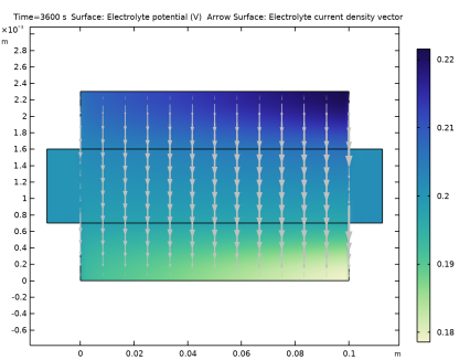
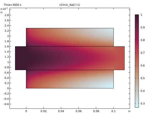
In the Model Builder window, expand the Results > Electrode Potential with Respect to Ground (tcd) node, then click Electrode Potential with Respect to Ground (tcd).
|
|
2
|
|
3
|
|
1
|
|
2
|
|
3
|
|
1
|
|
2
|
|
3
|
|
4
|
|
1
|
|
2
|
|
1
|
|
2
|
|
3
|
|
1
|
|
2
|
|
3
|
|
4
|
|
5
|
|
7
|
|
8
|
|
9
|
|
1
|
|
2
|
|
3
|
|
1
|
|
2
|
|
3
|
|
1
|
|
2
|
|
3
|
|
4
|
|
5
|
|
7
|
|
8
|
|
9
|
|
1
|
|
2
|
|
3
|
|
1
|
|
2
|
|
3
|
|
1
|
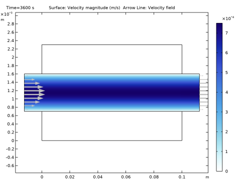
In the Settings window for Arrow Line, click Replace Expression in the upper-right corner of the Expression section. From the menu, choose Component 1 (comp1) > Brinkman Equations > Velocity and pressure > u,v - Velocity field.
|
|
2
|
|
3
|
|
4
|
Locate the Coloring and Style section.
|
|
5
|
|
6
|
|
1
|
|
2
|
|
3
|
Click
|
|
4
|
|
5
|
Click OK.
|
|
6
|
|
1
|
|
2
|
|
3
|
|
1
|
|
2
|
|
3
|
|
1
|
In the Model Builder window, expand the Domain ODEs and DAEs: Micropore Electrolyte Potential node, then click Surface 1.
|
|
2
|
|
3
|
|
1
|
|
2
|
|
3
|
|
1
|
In the Model Builder window, expand the Domain ODEs and DAEs: Attractive Potential node, then click Surface 1.
|
|
2
|
|
3
|
|
1
|
|
2
|
|
3
|
|
1
|
|
2
|
|
3
|
|
4
|
|
5
|
|
1
|
|
2
|
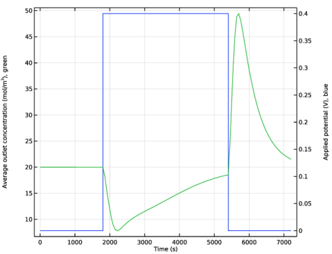
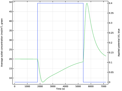
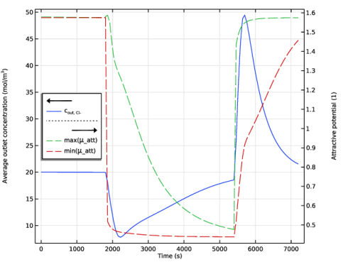
In the Settings window for 1D Plot Group, type Mixing-Cup Average Outlet Salt Concentration in the Label text field.
|
|
3
|
|
4
|
Locate the Plot Settings section.
|
|
5
|
Select the y-axis label checkbox. In the associated text field, type Average outlet concentration (mol/m<sup>3</sup>), green.
|
|
6
|
Select the Two y-axes checkbox.
|
|
7
|
Select the Secondary y-axis label checkbox. In the associated text field, type Applied potential (V), blue.
|
|
8
|
|
1
|
|
2
|
|
3
|
|
4
|
Click Replace Expression in the upper-right corner of the y-Axis Data section. From the menu, choose Component 1 (comp1) > Tertiary Current Distribution, Nernst–Planck > Load Cycle 1 > tcd.lc1.E_app - Applied voltage - V.
|
|
1
|
|
2
|
|
4
|
|
1
|
In the Model Builder window, right-click Mixing-Cup Average Outlet Salt Concentration and choose Duplicate.
|
|
2
|
|
3
|
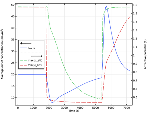
In the Settings window for 1D Plot Group, type Mixing-Cup Average Outlet Salt Concentration and mu in the Label text field.
|
|
4
|
Locate the Plot Settings section. In the y-axis label text field, type Average outlet concentration (mol/m<sup>3</sup>).
|
|
5
|
|
6
|
|
7
|
|
1
|
|
2
|
|
1
|
In the Settings window for Global, type Max and min \mu_att, upper electrode in the Label text field.
|
|
2
|
|
3
|
Locate the y-Axis Data section. In the table, enter the following settings:
|
|
4
|
Click to expand the Coloring and Style section. Find the Line style subsection. From the Line list, choose Dashed.
|
|
5
|
|
1
|
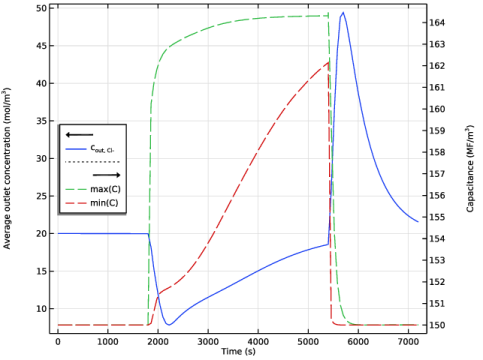
In the Model Builder window, right-click Mixing-Cup Average Outlet Salt Concentration and mu and choose Duplicate.
|
|
2
|
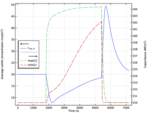
In the Settings window for 1D Plot Group, type Mixing-Cup Average Outlet Salt Concentration and C in the Label text field.
|
|
3
|
Locate the Plot Settings section. In the Secondary y-axis label text field, type Capacitance (MF/m<sup>3</sup>).
|
|
1
|
In the Model Builder window, expand the Mixing-Cup Average Outlet Salt Concentration and C node, then click Max and min \mu_att, upper electrode.
|
|
2
|
|
3
|
Locate the y-Axis Data section. In the table, enter the following settings:
|
|
4
|
|
1
|
|
2
|
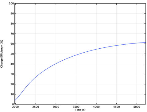
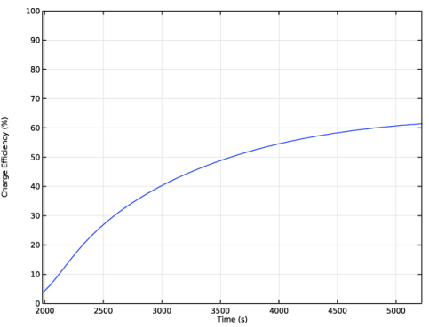
In the Settings window for Evaluation Group, type Evaluation Group: Charge Efficiency in the Label text field.
|
|
1
|
|
2
|
In the Settings window for Global Evaluation, type Cumulative Amount of Salt Entering the Cell in the Label text field.
|
|
3
|
Locate the Expressions section. In the table, enter the following settings:
|
|
4
|
|
5
|
Select the Cumulative checkbox.
|
|
1
|
In the Settings window for Line Integration, type Cumulative Amount of Salt Exiting the Cell in the Label text field.
|
|
3
|
|
5
|
|
6
|
Select the Cumulative checkbox.
|
|
1
|
|
3
|
|
5
|
|
6
|
Select the Cumulative checkbox.
|
|
1
|
|
2
|
|
3
|
|
4
|
|
5
|
|
6
|
|
1
|
Go to the Evaluation Group: Charge Efficiency window.
|
|
2
|
Click the Table Graph button in the window toolbar.
|
|
1
|
|
2
|
|
3
|
|
4
|
|
1
|
|
2
|
|
3
|
Locate the Plot Settings section.
|
|
4
|
|
5
|
|
6
|
|
7
|
|
8
|
|
9
|
|
10
|
|
1
|
|
2
|
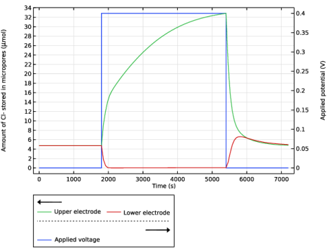
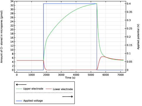
In the Settings window for 1D Plot Group, type Amount of Cl- Stored in Micropores in the Label text field.
|
|
3
|
|
4
|
Locate the Plot Settings section.
|
|
5
|
|
6
|
Select the y-axis label checkbox. In the associated text field, type Amount of Cl- stored in micropores (\mu mol).
|
|
7
|
Select the Two y-axes checkbox.
|
|
8
|
Select the Secondary y-axis label checkbox. In the associated text field, type Applied potential (V).
|
|
9
|
|
10
|
|
1
|
|
2
|
|
3
|
|
4
|
Click Replace Expression in the upper-right corner of the y-Axis Data section. From the menu, choose Component 1 (comp1) > Tertiary Current Distribution, Nernst–Planck > Load Cycle 1 > tcd.lc1.E_app - Applied voltage - V.
|
|
1
|
|
2
|
|
4
|