PDF

Adsorption–Desorption Voltammetry
Introduction
For an electrochemical reaction to occur, the reacting species usually needs to adsorb to the electrode surface before undergoing reduction or oxidation, after which the resulting product species desorbs back into the electrolyte.
If the rate of adsorption or desorption is slow in comparison to the electrochemical charge transfer step, the adsorption–desorption phenomena may have to be accounted for in a model.
This example investigates the impact of various kinetic parameters for adsorption, desorption and electron transfer when performing cyclic voltammetry on a planar disk electrode.
The examples replicates the results of Ref. 1.
Model Definition
The model defines diffusion (by Fick’s law) of an electrolyte species in a 1D geometry between x = 0 and x = L, and the local mass balances of two surface species at an electrode surface located at x = 0.
At the electrode boundary (x = 0) the electrolyte species A may adsorb according to
The adsorbed species Aads may then undergo reduction to form Bads in a charge transfer reaction according to
Langmuir isotherms are used for describing the kinetics, with the adsorption rate defined as
where ka1 is the adsorption rate constant, cA the electrolyte concentration of species A, the electrode surface coverage of species Aads, the electrode surface coverage of species Bads, and kd1 the desorption rate constant.
The charge transfer reaction is defined as
where k0 is the charge transfer rate constant, Γ the density of surface sites at the electrode, F Faraday’s constant, R the molar gas constant, T the temperature, and η the overpotential.
The overpotential η is defined as
where E is the electrode potential and E0 the formal potential.
The model is solved in a time-dependent simulation, ramping the potential from +0.5 V to 0.5 V and back, simulating a cyclic voltammogram.
When evaluating the voltammograms below, the total electrode current is defined as
where rd is the radius of the disk electrode.
The initial surface coverage of Aads is set to  = 0, defining a situation where the cyclic voltammogram is recorded shortly after immersing the electrode in the electrolyte.
Two dimensionless parameters, K' and k0', are altered in a parametric sweep. They are defined as
and
respectively. A high K' value hence represents a fast adsorption/slow desorption case, whereas a high k0' value represents a case featuring fast charge transfer. The simulated cases are described in Table 1.
K'
k0'
10-5
10-2
Results and Discussion
Figure 1 shows the voltammograms for the three simulated cases. Case 1, with fast adsorption and fast kinetics results in a voltammogram fairly symmetric and centered around E = 0 V. The total integral of the reduction current (negative peak) is significantly lower than the integrated oxidation current (positive peak). This is a result of the adsorption–desorption reaction not being in equilibrium ( = 0) when the simulation is started.
Figure 1: Cyclic voltammograms for the three investigated cases of 1) fast adsorption and charge transfer (blue), 2) slow adsorption and fast charge transfer (green), and 3) fast adsorption and slow charge transfer (red).
Case 2, with slower adsorption, features a limiting reduction current at E < −0.1 V, whereas the oxidation peak is fairly similar to that of Case 1.
Case 3, with slower charge transfer kinetics, features a more pronounced separation between the peaks.
More insights may be gained by inspecting the electrode surface coverages of Aads and Bads and the electrolyte concentration of species A at the electrode surface, as is shown in Figure 2 to Figure 4.
Figure 2: Surface coverages of species Aads and Bads and the concentration of A at the electrode surface for case 1) fast adsorption and fast charge transfer.
Figure 3: Surface coverages of species Aads and Bads and the concentration of A at the electrode surface for case 2) slow adsorption and fast charge transfer.
Figure 4: Surface coverages of species Aads and Bads and the concentration of A at the electrode surface for case 3) fast adsorption and slow charge transfer.
Reference
1. F. Chevallier, O. Klymenko, L. Jiang, T. Jones, and R. Compton, “Mathematical modelling and numerical simulation of adsorption processes at microdisk electrodes” J. Electroanal. Chem., vol. 574, pp. 217–237, 2005.
Application Library path: Electrochemistry_Module/Electroanalysis/adsorption_desorption_voltammetry
Modeling Instructions
From the File menu, choose New.
New
In the New window, click  Model Wizard.
Model Wizard
1
In the Model Wizard window, click  1D.
2
In the Select Physics tree, select Electrochemistry > Electroanalysis (tcd).
3
Click Add.
This model will model the transport of one species only (species A) in the electrolyte.
4
In the Number of species text field, type 1.
5
In the Concentrations (mol/m³) table, enter the following settings:
6
Click  Study.
7
In the Select Study tree, select Preset Studies for Selected Physics Interfaces > Cyclic Voltammetry.
8
Global Definitions
Parameters 1
1
In the Model Builder window, under Global Definitions click Parameters 1.
2
In the Settings window for Parameters, locate the Parameters section.
3
Click  Load from File.
4
Geometry 1
Interval 1 (i1)
1
In the Model Builder window, under Component 1 (comp1) right-click Geometry 1 and choose Interval.
2
In the Settings window for Interval, locate the Interval section.
3
4
Click  Build All Objects.
Electroanalysis (tcd)
1
In the Model Builder window, under Component 1 (comp1) click Electroanalysis (tcd).
2
In the Settings window for Electroanalysis, locate the Cross-Sectional Area section.
3
In the Ac text field, type A_electrode.
Electrolyte 1
1
In the Model Builder window, under Component 1 (comp1) > Electroanalysis (tcd) click Electrolyte 1.
2
In the Settings window for Electrolyte, locate the Diffusion section.
3
In the DcA text field, type D_A.
Initial Values 1
1
In the Model Builder window, click Initial Values 1.
2
In the Settings window for Initial Values, locate the Initial Values section.
3
In the cA text field, type c_A_bulk.
Electrode Surface 1
1
In the Physics toolbar, click  Boundaries and choose Electrode Surface.
You will only work with one electrode surface. Select the boundary to work with by clicking on it in the graphics window on the right:
2
3
In the Settings window for Electrode Surface, click to expand the Adsorbing–Desorbing Species section.
4
In the Γs text field, type Gamma.
At the electrode surface, we will model the surface coverages of two species (species A_ads and B_ads).
5
6
7
8
9
Locate the Electrode Phase Potential Condition section. From the Electrode phase potential condition list, choose Cyclic voltammetry.
10
In the Linear sweep rate text field, type nu.
11
In the Vertex potential 1 text field, type E_start.
12
In the Vertex potential 2 text field, type E_vertex.
Electrode Reaction 1
1
In the Model Builder window, click Electrode Reaction 1.
2
In the Settings window for Electrode Reaction, locate the Model Input section.
3
From the T list, choose User defined. In the associated text field, type T.
In the one-electron electrode charge transfer reaction, A_ads gets reduced to form B_ads. The electrolyte species A does not participate in the reaction.
4
Locate the Stoichiometric Coefficients section. In the Stoichiometric coefficients for adsorbing–desorbing species: table, enter the following settings:
5
Locate the Equilibrium Potential section. From the Eeq list, choose User defined. In the associated text field, type E_0.
6
Locate the Electrode Kinetics section. From the Kinetics expression type list, choose Concentration dependent kinetics.
7
In the i0 text field, type k0*F_const*Gamma.
8
In the CR text field, type tcd.theta_es1_B_ads.
9
In the CO text field, type tcd.theta_es1_A_ads.
tcd.theta_es1_A_ads and tcd.theta_es1_B_ads are the variable names for the surface coverage of A_ads and B_ads, respectively.
Definitions
Now the adsorption-desorption rate and the reaction, involving species A, A_ads and the amount of free sites, will be defined.
Variables 1
1
In the Model Builder window, under Component 1 (comp1) right-click Definitions and choose Variables.
Define a variable expression for the adsorption rate as follows:
2
In the Settings window for Variables, locate the Variables section.
3
In the expression above, tcd.thetafree_es1 is the surface fraction of free sites and c_A is the electrolyte concentration of species A. The values of the rate constants ka1 and kd1 are specified in the Parameters node by the text file you imported earlier.
Electroanalysis (tcd)
Electrode Surface 1
In the Model Builder window, under Component 1 (comp1) > Electroanalysis (tcd) click Electrode Surface 1.
Nonfaradaic Reactions 1
1
In the Physics toolbar, click  Attributes and choose Nonfaradaic Reactions.
2
In the Settings window for Nonfaradaic Reactions, locate the Reaction Rate section.
3
Select the Species c_A checkbox.
4
In the R0,cA text field, type -r_ads.
5
In the Reaction rate for adsorbing–desorbing species table, enter the following settings:
Electrode Surface 1
In the Model Builder window, click Electrode Surface 1.
Initial Values for Adsorbing–Desorbing Species 1
1
In the Physics toolbar, click  Attributes and choose Initial Values for Adsorbing–Desorbing Species.
2
In the Settings window for Initial Values for Adsorbing–Desorbing Species, locate the Initial Values for Adsorbing–Desorbing Species section.
3
The value of theta_A_init is 0, but may changed later in Parameters.
Mesh 1
To edit the mesh and get a very finely resolved mesh close to the electrode surface, proceed with these steps:
1
In the Model Builder window, under Component 1 (comp1) right-click Mesh 1 and choose Edit Physics-Induced Sequence.
Size
1
In the Model Builder window, under Component 1 (comp1) > Mesh 1 click Size.
2
In the Settings window for Size, locate the Element Size section.
3
Click the Custom button.
4
Locate the Element Size Parameters section. In the Maximum element size text field, type L/10.
5
In the Maximum element growth rate text field, type 1.1.
Size 1
1
In the Model Builder window, click Size 1.
2
In the Settings window for Size, locate the Element Size section.
3
Click the Custom button.
4
Locate the Element Size Parameters section.
5
Select the Maximum element size checkbox. In the associated text field, type L/10000.
Edge 1
In the Model Builder window, right-click Edge 1 and choose Build All.
Study 1
The model is now ready for solving. Add a parametric sweep to solve for three different sets of parameters.
Parametric Sweep
1
In the Study toolbar, click  Parametric Sweep.
2
In the Settings window for Parametric Sweep, locate the Study Settings section.
3
4
K_prime is a dimensionless parameter representing the ratio of the adsorption versus the desorption rate.
5
6
k_0_prime is a dimensionless parameter representing the charge transfer rate constant.
With the above settings you will now compute and compare: 1) a base case, 2) a reaction limited by adsorption and 3) a case limited by slow charge transfer.
7
In the Study toolbar, click  Compute.
Results
Cyclic Voltammograms (tcd)
The following will modify the automatically created voltammogram plot.
Global 1
1
In the Model Builder window, expand the Cyclic Voltammograms (tcd) node, then click Global 1.
2
In the Settings window for Global, click to expand the Legends section.
Polish the legend as follows:
3
From the Legends list, choose Evaluated.
4
In the Legend text field, type K'=eval(K_prime), k<sub>0</sub>'=eval(k_0_prime).
Compare the plot with Figure 1.
Surface Coverages and Concentration
Plot the surface coverages of A_ads and B_ads, as well as the electrolyte concentration of A, at the electrode surface for the three cases as follows:
1
In the Results toolbar, click  1D Plot Group.
2
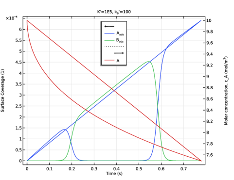
In the Settings window for 1D Plot Group, type Surface Coverages and Concentration in the Label text field.
3
Locate the Data section. From the Dataset list, choose Study 1/Parametric Solutions 1 (sol2).
4
From the Parameter selection (K_prime, k_0_prime) list, choose From list.
5
In the Parameter values (K_prime,k_0_prime) list box, select 1: K_prime=1E5, k_0_prime=100.
Point Graph 1
1
Right-click Surface Coverages and Concentration and choose Point Graph.
Select the leftmost boundary in the graphics window.
2
3
In the Settings window for Point Graph, click Replace Expression in the upper-right corner of the y-Axis Data section. From the menu, choose Component 1 (comp1) > Electroanalysis > Adsorbing–desorbing species > Surface coverage of adsorbing–desorbing species > tcd.theta_es1_A_ads - Surface coverage of adsorbing–desorbing species, 1-component.
4
Click to expand the Legends section. Select the Show legends checkbox.
5
From the Legends list, choose Manual.
6
7
In the Surface Coverages and Concentration toolbar, click  Plot.
Point Graph 2
1
Right-click Point Graph 1 and choose Duplicate.
2
In the Settings window for Point Graph, click Replace Expression in the upper-right corner of the y-Axis Data section. From the menu, choose Component 1 (comp1) > Electroanalysis > Adsorbing–desorbing species > Surface coverage of adsorbing–desorbing species > tcd.theta_es1_B_ads - Surface coverage of adsorbing–desorbing species, 2-component.
3
Locate the Legends section. In the table, enter the following settings:
4
In the Surface Coverages and Concentration toolbar, click  Plot.
Point Graph 3
1
Right-click Point Graph 2 and choose Duplicate.
2
In the Settings window for Point Graph, click Replace Expression in the upper-right corner of the y-Axis Data section. From the menu, choose Component 1 (comp1) > Electroanalysis > Species c_A > c_A - Molar concentration, c_A - mol/m³.
3
Locate the Legends section. In the table, enter the following settings:
Surface Coverages and Concentration
To polish the title, y-axis settings and legend position, proceed as follows:
1
In the Model Builder window, click Surface Coverages and Concentration.
2
In the Settings window for 1D Plot Group, click to expand the Title section.
3
From the Title type list, choose Manual.
4
In the Title text area, type K'=eval(K_prime), k<sub>0</sub>'=eval(k_0_prime).
5
Locate the Plot Settings section.
6
Select the y-axis label checkbox. In the associated text field, type Surface Coverage (1).
7
Select the Two y-axes checkbox.
8
In the table, select the Plot on secondary y-axis checkbox for Point Graph 3.
9
Locate the Legend section. From the Position list, choose Upper middle.
10
In the Surface Coverages and Concentration toolbar, click  Plot.
Compare the plot with Figure 2.
11
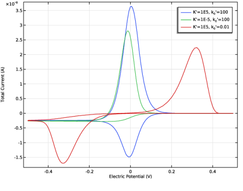
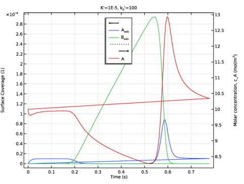
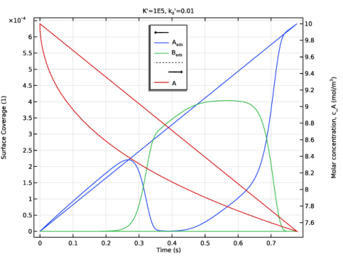
Locate the Data section. In the Parameter values (K_prime,k_0_prime) list box, select 2: K_prime=1E-5, k_0_prime=100.
12
In the Surface Coverages and Concentration toolbar, click  Plot.
Compare the plot with Figure 3.
13
In the Parameter values (K_prime,k_0_prime) list box, select 3: K_prime=1E5, k_0_prime=0.01.
14
In the Surface Coverages and Concentration toolbar, click  Plot.
Compare the plot with Figure 4.