|
|
|


|
1
|
|
2
|
In the Application Libraries window, select Corrosion Module > Galvanic Corrosion > galvanic_corrosion_with_deformation in the tree.
|
|
3
|
Click
|
|
1
|
|
2
|
Go to the Add Physics window.
|
|
3
|
|
4
|
|
5
|
In the Concentrations (mol/m³) table, enter the following settings:
|
|
6
|
Click the Add to Selection button in the window toolbar.
|
|
7
|
|
8
|
Click the Add to Selection button in the window toolbar.
|
|
9
|
|
1
|
|
2
|
|
3
|
Click
|
|
4
|
Browse to the model’s Application Libraries folder and double-click the file under_deposit_corrosion_parameters.txt.
|
|
1
|
|
2
|
|
3
|
|
1
|
|
2
|
|
3
|
Click
|
|
4
|
Browse to the model’s Application Libraries folder and double-click the file under_deposit_corrosion_variables.txt.
|
|
1
|
|
2
|
|
3
|
|
5
|
|
6
|
|
7
|
Select the Use source map checkbox.
|
|
8
|
|
9
|
|
1
|
|
2
|
|
3
|
Clear the Convection checkbox.
|
|
4
|
Select the Migration in electric field checkbox.
|
|
1
|
In the Model Builder window, under Component 1 (comp1) > Transport of Diluted Species (tds) click Species Charges.
|
|
2
|
|
3
|
|
4
|
|
1
|
|
2
|
|
3
|
|
4
|
|
5
|
|
1
|
|
2
|
|
3
|
|
1
|
|
3
|
|
4
|
|
5
|
|
1
|
|
3
|
|
4
|
Select the Species cOH checkbox.
|
|
5
|
|
1
|
|
1
|
In the Model Builder window, expand the Electrode Surface Coupling 1 node, then click Reaction Coefficients 1.
|
|
2
|
|
3
|
|
4
|
|
5
|
|
1
|
|
1
|
In the Model Builder window, expand the Electrode Surface Coupling 2 node, then click Reaction Coefficients 1.
|
|
2
|
|
3
|
|
4
|
|
5
|
|
1
|
|
1
|
|
2
|
|
3
|
|
4
|
|
5
|
|
1
|
|
2
|
|
3
|
|
1
|
|
2
|
|
3
|
Click
|
|
4
|
|
5
|
Click OK.
|
|
1
|
|
1
|
In the Model Builder window, expand the Secondary Current Distribution (cd) node, then click Electrolyte 1.
|
|
2
|
|
3
|
|
1
|
|
2
|
|
1
|
|
2
|
|
3
|
|
4
|
|
1
|
|
2
|
|
3
|
|
1
|
|
2
|
|
3
|
|
5
|
|
6
|
|
7
|
|
1
|
In the Model Builder window, expand the Study 1 node, then click Step 1: Current Distribution Initialization.
|
|
2
|
In the Settings window for Current Distribution Initialization, locate the Physics and Variables Selection section.
|
|
3
|
In the Solve for column of the table, under Component 1 (comp1), clear the checkbox for Deformed Geometry.
|
|
4
|
|
1
|
|
2
|
|
3
|
|
4
|
Locate the Coloring and Style section. Find the Point style subsection. From the Arrow length list, choose Normalized.
|
|
1
|
|
2
|
|
3
|
|
4
|
|
5
|
|
1
|
|
2
|
|
3
|
|
1
|
|
2
|
|
3
|
|
4
|
|
5
|
|
1
|
|
2
|
|
3
|
|
4
|
|
1
|
|
2
|
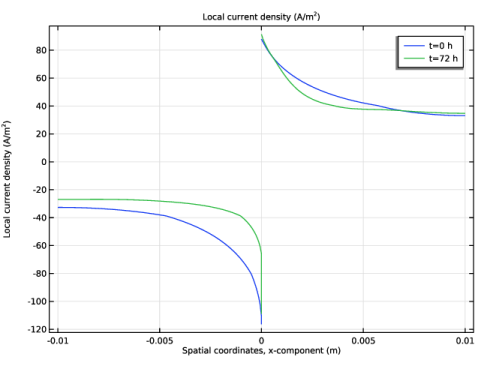
In the Settings window for 1D Plot Group, type Local Current Density Change in the Label text field.
|
|
3
|
|
1
|
|
2
|
|
3
|
|
4
|
|
1
|
|
2
|
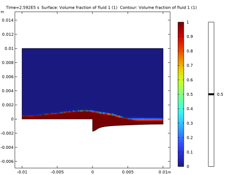
In the Settings window for Surface, click Replace Expression in the upper-right corner of the Expression section. From the menu, choose Component 1 (comp1) > Level Set > ls.Vf1 - Volume fraction of fluid 1 - 1.
|
|
3
|
|
1
|
|
2
|
In the Settings window for Contour, click Replace Expression in the upper-right corner of the Expression section. From the menu, choose Component 1 (comp1) > Level Set > ls.Vf1 - Volume fraction of fluid 1 - 1.
|
|
3
|
|
4
|
|
5
|
|
6
|
|
7
|
|
8
|