|
|
|

|
1
|
|
2
|
|
3
|
Click Add.
|
|
4
|
In the Select Physics tree, select Electrochemistry > Primary and Secondary Current Distribution > Secondary Current Distribution (cd).
|
|
5
|
Click Add.
|
|
6
|
Click
|
|
7
|
|
8
|
Click
|
|
1
|
|
2
|
|
3
|
|
4
|
|
1
|
|
2
|
|
3
|
|
4
|
|
5
|
|
6
|
|
1
|
|
2
|
Select the object r1 only.
|
|
3
|
|
4
|
|
5
|
Select the object e1 only.
|
|
1
|
|
2
|
|
3
|
|
4
|
Click
|
|
5
|
|
1
|
|
2
|
|
3
|
Click
|
|
4
|
Browse to the model’s Application Libraries folder and double-click the file stress_corrosion_parameters.txt.
|
|
1
|
|
2
|
|
3
|
|
4
|
Click
|
|
5
|
Browse to the model’s Application Libraries folder and double-click the file stress_corrosion_variables.txt.
|
|
1
|
|
2
|
|
3
|
|
4
|
Click
|
|
5
|
Browse to the model’s Application Libraries folder and double-click the file stress_corrosion_stress_strain_curve_interpolation.txt.
|
|
6
|
Locate the Interpolation and Extrapolation section. From the Interpolation list, choose Piecewise cubic.
|
|
7
|
|
8
|
In the Function table, enter the following settings:
|
|
1
|
|
2
|
|
4
|
Click
|
|
1
|
|
2
|
|
3
|
|
1
|
|
2
|
Go to the Add Material window.
|
|
3
|
|
4
|
Click the Add to Component button in the window toolbar.
|
|
5
|
|
1
|
|
3
|
Click
|
|
5
|
Locate the Material Contents section. In the table, set the following property values:
|
|
1
|
In the Model Builder window, under Component 1 (comp1) > Solid Mechanics (solid) click Initial Values 1.
|
|
2
|
|
3
|
Specify the u vector as
|
|
1
|
|
1
|
|
3
|
|
4
|
|
5
|
|
1
|
|
3
|
|
4
|
|
1
|
|
1
|
In the Model Builder window, under Component 1 (comp1) > Secondary Current Distribution (cd) click Electrolyte 1.
|
|
2
|
|
3
|
|
1
|
|
2
|
|
3
|
|
1
|
|
3
|
|
4
|
|
1
|
|
1
|
|
2
|
|
3
|
|
4
|
Locate the Electrode Kinetics section. From the Kinetics expression type list, choose Anodic Tafel equation.
|
|
5
|
|
6
|
|
1
|
|
2
|
|
3
|
|
4
|
Locate the Electrode Kinetics section. From the Kinetics expression type list, choose Cathodic Tafel equation.
|
|
5
|
|
6
|
|
1
|
|
1
|
|
2
|
|
3
|
|
5
|
|
6
|
Locate the Element Size Parameters section.
|
|
7
|
|
1
|
|
2
|
|
3
|
|
5
|
|
6
|
Locate the Element Size Parameters section.
|
|
7
|
|
8
|
Click
|
|
1
|
|
2
|
|
1
|
|
2
|
|
3
|
Click
|
|
1
|
|
2
|
|
3
|
In the Solve for column of the table, under Component 1 (comp1), clear the checkbox for Secondary Current Distribution (cd).
|
|
1
|
|
2
|
|
3
|
In the Solve for column of the table, under Component 1 (comp1), clear the checkbox for Solid Mechanics (solid).
|
|
4
|
|
5
|
|
6
|
|
7
|
|
8
|
Clear the Generate default plots checkbox.
|
|
9
|
|
1
|
|
2
|
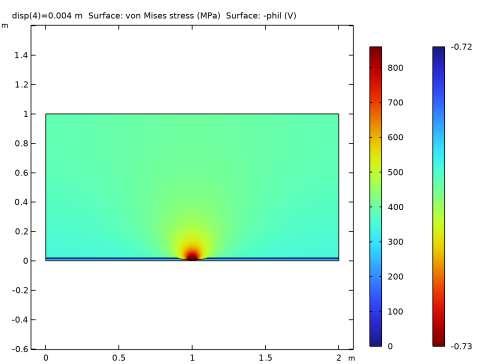
In the Settings window for 2D Plot Group, type Corrosion Potential and von Mises Stress in the Label text field.
|
|
3
|
Locate the Data section. From the Dataset list, choose Study: Stationary Parametric/Parametric Solutions 1 (sol3).
|
|
1
|
|
2
|
In the Settings window for Surface, click Replace Expression in the upper-right corner of the Expression section. From the menu, choose Component 1 (comp1) > Solid Mechanics > Stress > solid.misesGp - von Mises stress - N/m².
|
|
3
|
|
1
|
|
2
|
|
3
|
|
4
|
|
5
|
|
6
|
|
7
|
|
8
|
|
9
|
|
1
|
|
2
|
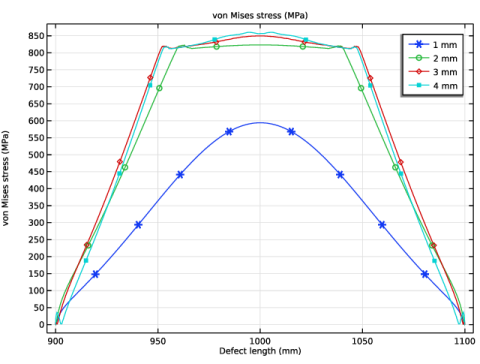
In the Settings window for 1D Plot Group, type von Mises Stress, Parametric in the Label text field.
|
|
3
|
Locate the Data section. From the Dataset list, choose Study: Stationary Parametric/Parametric Solutions 1 (sol3).
|
|
4
|
Locate the Plot Settings section.
|
|
5
|
|
1
|
|
3
|
In the Settings window for Line Graph, click Replace Expression in the upper-right corner of the y-Axis Data section. From the menu, choose Component 1 (comp1) > Solid Mechanics > Stress > solid.misesGp - von Mises stress - N/m².
|
|
4
|
|
5
|
|
6
|
|
7
|
|
8
|
Click to expand the Coloring and Style section. Find the Line markers subsection. From the Marker list, choose Cycle.
|
|
9
|
|
10
|
|
11
|
|
12
|
|
13
|
|
1
|
|
2
|
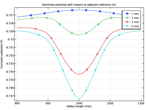
In the Settings window for 1D Plot Group, type Corrosion Potential, Parametric in the Label text field.
|
|
3
|
Locate the Plot Settings section.
|
|
4
|
|
1
|
In the Model Builder window, expand the Corrosion Potential, Parametric node, then click Line Graph 1.
|
|
2
|
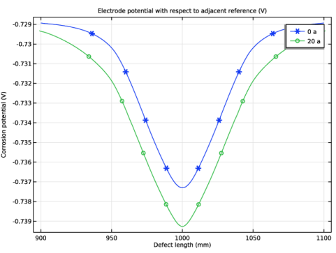
In the Settings window for Line Graph, click Replace Expression in the upper-right corner of the y-Axis Data section. From the menu, choose Component 1 (comp1) > Secondary Current Distribution > cd.Evsref - Electrode potential with respect to adjacent reference - V.
|
|
3
|
|
1
|
|
2
|
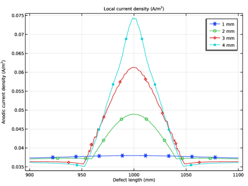
In the Settings window for 1D Plot Group, type Anodic Current Density, Parametric in the Label text field.
|
|
3
|
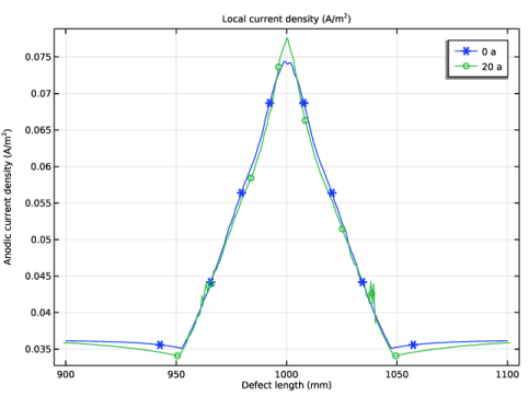
Locate the Plot Settings section. In the y-axis label text field, type Anodic current density (A/m<sup>2</sup>).
|
|
1
|
In the Model Builder window, expand the Anodic Current Density, Parametric node, then click Line Graph 1.
|
|
2
|
In the Settings window for Line Graph, click Replace Expression in the upper-right corner of the y-Axis Data section. From the menu, choose Component 1 (comp1) > Secondary Current Distribution > Electrode kinetics > cd.iloc_er1 - Local current density - A/m².
|
|
3
|
|
1
|
|
2
|
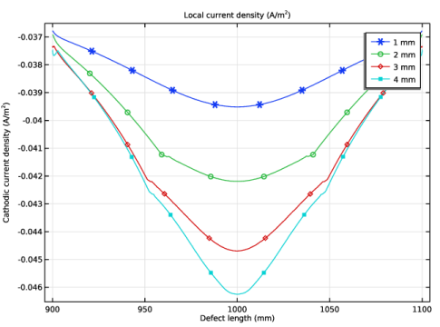
In the Settings window for 1D Plot Group, type Cathodic Current Density, Parametric in the Label text field.
|
|
3
|
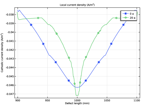
Locate the Plot Settings section. In the y-axis label text field, type Cathodic current density (A/m<sup>2</sup>).
|
|
1
|
In the Model Builder window, expand the Cathodic Current Density, Parametric node, then click Line Graph 1.
|
|
2
|
In the Settings window for Line Graph, click Replace Expression in the upper-right corner of the y-Axis Data section. From the menu, choose Component 1 (comp1) > Secondary Current Distribution > Electrode kinetics > cd.iloc_er2 - Local current density - A/m².
|
|
3
|
|
1
|
|
2
|
|
3
|
|
1
|
In the Model Builder window, under Component 1 (comp1) > Secondary Current Distribution (cd) click Internal Electrode Surface 1.
|
|
2
|
In the Settings window for Internal Electrode Surface, click to expand the Dissolving–Depositing Species section.
|
|
3
|
Click
|
|
1
|
|
2
|
|
3
|
In the Stoichiometric coefficients for dissolving–depositing species: table, enter the following settings:
|
|
1
|
|
2
|
|
3
|
|
4
|
Locate the Nondeforming Boundary section. From the Boundary condition list, choose Zero normal displacement.
|
|
1
|
In the Physics toolbar, click
|
|
2
|
|
3
|
|
1
|
|
2
|
|
3
|
In the Solve for column of the table, under Component 1 (comp1), clear the checkbox for Deformed Geometry.
|
|
4
|
In the Solve for column of the table, under Component 1 (comp1) > Multiphysics, clear the checkboxes for Nondeforming Boundary 1 (ndbdg1) and Deforming Electrode Surface 1 (desdg1).
|
|
1
|
|
2
|
Go to the Add Study window.
|
|
3
|
|
4
|
Click the Add Study button in the window toolbar.
|
|
5
|
|
1
|
|
2
|
|
3
|
|
4
|
Click to expand the Values of Dependent Variables section. Find the Initial values of variables solved for subsection. From the Settings list, choose User controlled.
|
|
5
|
|
6
|
|
7
|
|
8
|
|
9
|
|
10
|
|
1
|
|
2
|
|
3
|
In the Model Builder window, expand the Study: Transient, Deformed Geometry > Solver Configurations > Solution 8 (sol8) > Time-Dependent Solver 1 node, then click Fully Coupled 1.
|
|
4
|
|
5
|
|
6
|
|
1
|
|
2
|
|
3
|
Locate the Data section. From the Dataset list, choose Study: Transient, Deformed Geometry/Solution 8 (sol8).
|
|
4
|
|
5
|
|
1
|
|
3
|
|
4
|
|
5
|
|
6
|
|
7
|
|
8
|
|
1
|
|
2
|
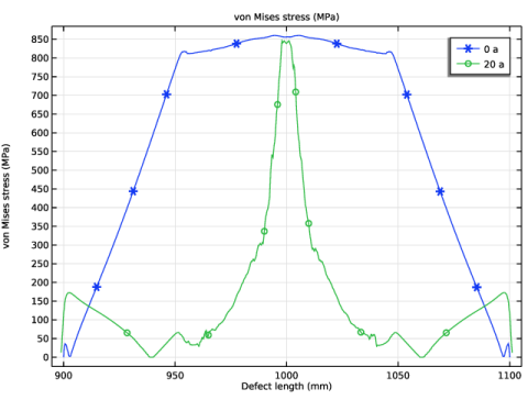
In the Settings window for 1D Plot Group, type von Mises Stress, Deformed Geometry in the Label text field.
|
|
3
|
Locate the Data section. From the Dataset list, choose Study: Transient, Deformed Geometry/Solution 8 (sol8).
|
|
4
|
|
5
|
|
1
|
In the Model Builder window, expand the von Mises Stress, Deformed Geometry node, then click Line Graph 1.
|
|
2
|
|
3
|
|
4
|
|
1
|
|
2
|
In the Settings window for 1D Plot Group, type Corrosion Potential, Deformed Geometry in the Label text field.
|
|
3
|
Locate the Data section. From the Dataset list, choose Study: Transient, Deformed Geometry/Solution 8 (sol8).
|
|
4
|
|
5
|
|
1
|
In the Model Builder window, expand the Corrosion Potential, Deformed Geometry node, then click Line Graph 1.
|
|
2
|
|
3
|
|
4
|
|
1
|
|
2
|
In the Settings window for 1D Plot Group, type Anodic Current Density, Deformed Geometry in the Label text field.
|
|
3
|
Locate the Data section. From the Dataset list, choose Study: Transient, Deformed Geometry/Solution 8 (sol8).
|
|
4
|
|
5
|
|
1
|
In the Model Builder window, expand the Anodic Current Density, Deformed Geometry node, then click Line Graph 1.
|
|
2
|
|
3
|
|
4
|
|
1
|
|
2
|
In the Settings window for 1D Plot Group, type Cathodic Current Density, Deformed Geometry in the Label text field.
|
|
3
|
Locate the Data section. From the Dataset list, choose Study: Transient, Deformed Geometry/Solution 8 (sol8).
|
|
4
|
|
5
|
|
1
|
In the Model Builder window, expand the Cathodic Current Density, Deformed Geometry node, then click Line Graph 1.
|
|
2
|
|
3
|
|
4
|