|
|
|

|
1
|
|
2
|
In the Select Physics tree, select Electrochemistry > Primary and Secondary Current Distribution > Secondary Current Distribution (cd).
|
|
3
|
Click Add.
|
|
4
|
|
5
|
Click Add.
|
|
6
|
Click
|
|
7
|
In the Select Study tree, select Preset Studies for Selected Physics Interfaces > Level Set > Time Dependent with Phase Initialization.
|
|
8
|
Click
|
|
1
|
|
2
|
|
3
|
|
4
|
|
5
|
|
1
|
|
2
|
|
3
|
|
4
|
|
5
|
|
6
|
|
7
|
Click
|
|
8
|
|
1
|
|
2
|
|
3
|
|
4
|
Click
|
|
5
|
Browse to the model’s Application Libraries folder and double-click the file localized_corrosion_ls_microstructure.txt.
|
|
6
|
Click
|
|
7
|
Locate the Data Column Settings section. In the table, click to select the cell at row number 1 and column number 1.
|
|
8
|
|
10
|
|
12
|
|
13
|
|
14
|
Click
|
|
1
|
|
2
|
|
3
|
|
1
|
|
2
|
|
1
|
|
2
|
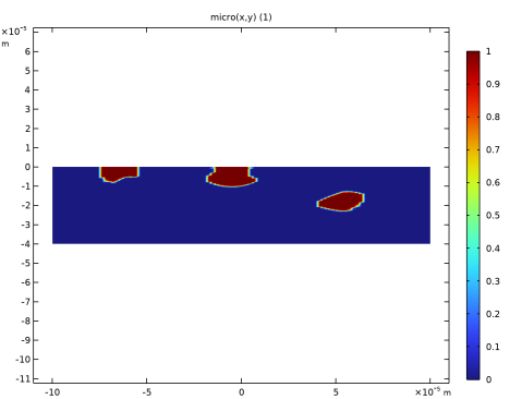
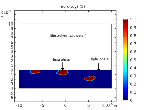
In the Settings window for 2D Plot Group, type 2D Plot Group : Cross-sectional microstructure in the Label text field.
|
|
3
|
|
1
|
|
2
|
|
3
|
Click
|
|
4
|
Browse to the model’s Application Libraries folder and double-click the file localized_corrosion_parameters.txt.
|
|
1
|
|
2
|
|
3
|
|
4
|
Click
|
|
5
|
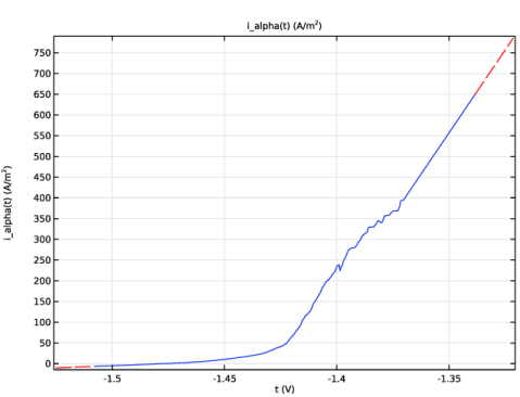
Browse to the model’s Application Libraries folder and double-click the file localized_corrosion_i_alpha.txt.
|
|
6
|
Locate the Interpolation and Extrapolation section. From the Interpolation list, choose Piecewise cubic.
|
|
7
|
|
8
|
|
9
|
In the Function table, enter the following settings:
|
|
10
|
Click
|
|
1
|
|
2
|
|
3
|
|
4
|
Click
|
|
5
|
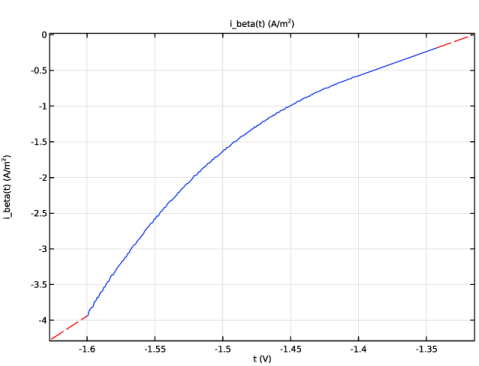
Browse to the model’s Application Libraries folder and double-click the file localized_corrosion_i_beta.txt.
|
|
6
|
Locate the Interpolation and Extrapolation section. From the Interpolation list, choose Piecewise cubic.
|
|
7
|
|
8
|
|
9
|
In the Function table, enter the following settings:
|
|
10
|
Click
|
|
1
|
|
2
|
Click in the Graphics window and then press Ctrl+A to select both domains.
|
|
1
|
|
2
|
|
3
|
Click
|
|
4
|
Browse to the model’s Application Libraries folder and double-click the file localized_corrosion_ls_variables.txt.
|
|
1
|
In the Model Builder window, under Component 1 (comp1) > Secondary Current Distribution (cd) click Electrolyte 1.
|
|
2
|
|
3
|
|
4
|
|
5
|
In the Show More Options dialog, in the tree, select the checkbox for the node Physics > Advanced Physics Options.
|
|
6
|
Click OK.
|
|
1
|
|
2
|
Click in the Graphics window and then press Ctrl+A to select both domains.
|
|
3
|
In the Settings window for Electrolyte Current Source, locate the Electrolyte Current Source section.
|
|
4
|
|
1
|
|
2
|
Click in the Graphics window and then press Ctrl+A to select both domains.
|
|
1
|
|
2
|
|
3
|
|
4
|
|
5
|
|
1
|
|
1
|
|
1
|
|
1
|
|
2
|
|
3
|
|
1
|
|
2
|
|
3
|
|
5
|
|
1
|
|
2
|
|
3
|
|
5
|
|
6
|
|
7
|
|
1
|
|
2
|
|
3
|
|
4
|
|
1
|
|
2
|
|
3
|
|
4
|
|
5
|
|
1
|
|
2
|
|
3
|
|
1
|
|
2
|
|
3
|
|
4
|
|
1
|
|
2
|
|
3
|
|
1
|
|
2
|
|
1
|
|
2
|
|
3
|
|
4
|
|
1
|
|
2
|
|
3
|
|
4
|
|
5
|
|
6
|
|
7
|
|
8
|