PDF

Corrosion Under an Evans Droplet
Introduction
An Evans droplet experiment is a century-old corrosion experiment for demonstrating oxygen transport-limited corrosion. A droplet of water is placed on a metal surface, and over time the surface features differences in the radial direction of the surface in terms of amount of corroded material and deposited corrosion products.
This tutorial model defines corrosion of an iron surface in contact with an aqueous sodium-chloride solution droplet in a surrounding atmosphere containing both carbon dioxide and oxygen. The model accounts for charge and mass transport of multiple species as well as iron dissolution, oxygen reduction, carbonic acid equilibria, iron hydrolysis, and precipitation of ferrous hydroxide and ferrous carbonate corrosion products.
The model computes the transient and spatial distributions of the various species within the droplet. A spatial gradient in pH is demonstrated and is attributed to the complex dynamic interplay between the dissolved iron, corrosion products, and dissolved atmospheric gases.
The model is based on several journal papers (Ref. 1Ref. 4).
Model Definition
Figure 1 shows the model geometry, defining an elliptical electrolyte droplet (with a 90° wetting angle) covering an iron metal surface. The geometry is defined in 2D with axial symmetry. As an assumption, the geometry is fixed throughout the simulation.
Figure 1: Model geometry.
The model is defined using the Aqueous Electrolyte Transport interface, solving for the electrolyte phase potential and the concentrations of the electrolyte species H+, OH-, Fe2+, FeOH+, Fe(OH)2(aq), FeCO3(aq), O2(aq), CO2(aq), H2CO3, HCO3-, CO32-, Na+, and Cl-.
Oxygen reduction occurs on the metal surface, which, due to limited oxygen diffusion, is more dominant toward the periphery of the droplet:
(1)
Iron is oxidized to counterbalance the oxygen reduction reaction:
(2)
Butler–Volmer electrode kinetics expressions are used for both the oxygen-reduction and iron-dissolution reactions. The combination of these two reactions gives rise to a mixed electrode potential of the metal surface.
Dissolved iron precipitates as ferrous hydroxide and ferrous carbonate corrosion products at the electrode surface due to the following reactions:
(3)
(4)
The reactions are defined as irreversible and precipitation takes place once the solubility product is exceeded. The corrosion products are said to cover the metallic surface and are assumed to only inhibit the metal dissolution, that is, the products passivate the iron. The corrosion-product coverage degree, θ, is computed with the expression
(5)
With the use of the above expression, the coverage can reach a maximum value of 1 with precipitation. ctot,s is the total molar amount per surface area of precipitated corrosion products and cavailable,s is the molar availability per surface area and monolayer for corrosion-product precipitation. The inhibition of the metal dissolution is modeled by multiplying the local current density of the metal dissolution reaction with the uncovered surface fraction, 1 − θ. Note that with the expression above more than cavailable,s needs to precipitate for full passivation.
Equilibrium Reactions
The following equilibrium reactions are accounted for in the electrolyte:
(6)
K1 through K7 are the equilibrium constants. Values have been chosen for temperatures near room temperature (293.15 K).
The water dissociation equilibrium reaction is built-in for the Aqueous Electrolyte Transport interface. All three carbonic acid reactions can be captured by adding the Carbonic Acid feature to the Electrolyte domain node. The Ampholyte feature is used to model the two iron hydrolysis reactions. Finally, the Complex Species feature allows for easy representation of the iron carbonate species. These equilibrium reaction features simultaneously calculate the concentration of all aqueous species based on equilibrium expressions, which are based on the reaction stoichiometry and the equilibrium constant Kk according to
(7)
where ci (SI unit: mol/m3) is the concentration of species i and vik is the stoichiometric coefficient of species i in reaction k.
As a result of the above equilibrium reactions, the gaseous CO2 dissolved at the droplet surface forms carbonic acid, which generally lowers the pH.
The model is solved using a time-dependent solver, simulating the transient and spatial evolution of the species considered for 300 seconds. Inward fluxes of O2 and CO2 are set relatively high at the upper droplet boundary facing the surrounding atmosphere such that the gas concentrations are approximately constant and equal to the saturation concentrations (O2(aq, sat) and CO2(aq, sat)) at the droplet surface.
Results and Discussion
Figure 2 shows the iron ion concentration distribution within the Evans droplet at 10 s (left) and 300 s (right). It can be seen that the concentration is lower within a ring expanding inward from the droplet periphery compared to the central parts of the droplet. At the 300 s, this ring with lower iron ion concentration has become approximately 1 mm wide.
Figure 2: Iron ion concentration distribution within the droplet at t = 10 s (left) and t = 300 s (right).
In Figure 3, the current density distributions and the corrosion-product coverage degree along the iron surface underneath the droplet at 300 s are displayed. The observed lower iron-ion concentration can be explained by the lower anodic metal-dissolution reaction which in turn is affected by the higher corrosion-product coverage degree at the same location. The short-time behavior in Figure 2 (left) is likewise explained by the coverage, which is less and means that the iron dissolution initially is present over almost the whole droplet covered surface.
The cathodic oxygen reduction is larger near the rim of the droplet due to limited oxygen transport, in combination with the limited electrolyte conductivity. The total current density shows that the anodic activity dominates the central parts of the droplet and the cathodic the periphery of the droplet.
Note that the droplet rim has a different behavior due to the acidifying CO2 from the atmosphere. This acidity counteracts any corrosion-product precipitation.
Figure 3: Iron dissolution, oxygen reduction, and total current density distributions along the iron surface at t = 300 s.
Figure 4 shows the CO2(aq) concentration distribution within the droplet at 10 s (left) and 300 s (right). It can be seen that the concentration is reduced close to the iron surface, since it is consumed in a homogeneous reaction.
Figure 4: CO2 concentration distribution within the droplet at t = 10 s (left) and t = 300 s (right).
Figure 5 shows the pH distribution within the droplet at 10 s (left) and 300 s (right). The pH changes over time are substantial. It can also be seen that the pH is increased in the vicinity of the metal surface, when compared to the pH closer to the droplet periphery. At the droplet rim, the pH is the lowest due to the CO2 in the atmosphere. The pH changes are generally attributed to the dissolution of iron atoms which need to be counter-balanced by hydroxide ions from water autoprotolysis. The iron hydrolysis is insufficient to acidify the electrolyte near the iron surface.
Figure 5: pH distribution within the droplet at t = 10 s (left) and t = 300 s (right).
Figure 6 shows the surface plot of precipitated corrosion products per area along the iron surface underneath the droplet and the streamline plot of the electrolyte current density over the droplet domain at 300 s. Most has precipitated in the ring region where the low iron-ion concentration is observed. A comparison with the coverage degree in Figure 3 indicates that ferrous carbonate almost exclusively makes up the coverage in that region. The access to carbonates in the form of carbonate ions near the droplet periphery is the main cause for this. The streamlines show the ionic current flow from the core toward the rim of the droplet.
Figure 6: Precipitated ferrous carbonate and ferrous oxide at the iron surface and streamline plot of the electrolyte current density at t = 300 s.
References
1. B.G. Koushik, N. Van den Steen, M.H. Mamme, Y. Van Ingelgem, and H. Terryn, “Review on modelling of corrosion under droplet electrolyte for predicting atmospheric corrosion rate,” J. Mater. Sci. Technol., vol. 62, pp. 254–267, 2021.
2. M. Nordsveen, S. Nesic, R. Nyborg, and A. Stangeland, “A Mechanistic Model for Carbon Dioxide Corrosion of Mild Steel in the Presence of Protective Iron Carbonate Films-Part 1: Theory and Verification,” Corrosion, vol. 59, no. 5, pp. 443–456, 2003.
3. P.L. Fosboel and K. Thomsen, “Review and recommended thermodynamic properties of FeCO3,” Corros. Sci. Technol., vol. 45, no. 2, pp. 115–135, 2010.
4. F.J. Millero, W. Yao, and J. Aicher, “The speciation of Fe(II) and Fe(III) in natural waters,” Marine Chemistry, vol. 50, pp. 21–39, 1995.
Application Library path: Corrosion_Module/Atmospheric_Corrosion/evans_droplet
Modeling Instructions
From the File menu, choose New.
New
In the New window, click  Model Wizard.
Model Wizard
1
In the Model Wizard window, click  2D Axisymmetric.
2
In the Select Physics tree, select Electrochemistry > Aqueous Electrolyte Transport (aqt).
3
Click Add.
4
Click  Study.
5
In the Select Study tree, select Preset Studies for Selected Physics Interfaces > Time Dependent with Initialization.
6
Global Definitions
Load the model parameters form a text file.
Parameters 1
1
In the Model Builder window, under Global Definitions click Parameters 1.
2
In the Settings window for Parameters, locate the Parameters section.
3
Click  Load from File.
4
Geometry 1
Ellipse 1 (e1)
The geometry consists of a sector of an ellipse.
1
In the Geometry toolbar, click  Ellipse.
2
In the Settings window for Ellipse, locate the Size and Shape section.
3
In the a-semiaxis text field, type a.
4
In the b-semiaxis text field, type b.
5
In the Sector angle text field, type 90.
6
Click  Build All Objects.
Definitions
Load the model variables from a text file. These include precipitation and passivation definitions.
Variables 1
1
In the Model Builder window, expand the Component 1 (comp1) > Definitions node.
2
Right-click Definitions and choose Local Variables.
3
In the Settings window for Variables, locate the Variables section.
4
Click  Load from File.
5
Aqueous Electrolyte Transport (aqt)
Electrolyte 1
Add all aqueous species in the Electrolyte feature. This includes Carbonic acid, which encompasses CO2 and all associated species, as well as the iron species, supporting electrolyte, and dissolved oxygen.
1
In the Model Builder window, under Component 1 (comp1) > Aqueous Electrolyte Transport (aqt) click Electrolyte 1.
Carbonic Acid 1
In the Physics toolbar, click  Attributes and choose Carbonic Acid.
Electrolyte 1
In the Model Builder window, click Electrolyte 1.
Ampholyte - Fe
1
In the Physics toolbar, click  Attributes and choose Ampholyte.
2
In the Settings window for Ampholyte, type Ampholyte - Fe in the Label text field.
3
Locate the Ampholyte section. In the Species name text field, type Fe.
4
5
In the z0 text field, type 0.
6
Locate the Diffusion and Migration section. In the D text field, type DFe.
Electrolyte 1
In the Model Builder window, click Electrolyte 1.
Uncharged Species - O2
1
In the Physics toolbar, click  Attributes and choose Uncharged Species.
2
In the Settings window for Uncharged Species, type Uncharged Species - O2 in the Label text field.
3
Locate the Uncharged Species section. In the Species name text field, type O2.
4
Locate the Diffusion section. In the D text field, type DO2.
Electrolyte 1
In the Model Builder window, click Electrolyte 1.
Fully Dissociated Species - Na
1
In the Physics toolbar, click  Attributes and choose Fully Dissociated Species.
2
In the Settings window for Fully Dissociated Species, type Fully Dissociated Species - Na in the Label text field.
3
Locate the Fully Dissociated Species section. In the Species name text field, type Na.
4
In the z text field, type zNa.
5
Locate the Diffusion and Migration section. In the D text field, type DNa.
Electrolyte 1
In the Model Builder window, click Electrolyte 1.
Fully Dissociated Species - Cl
1
In the Physics toolbar, click  Attributes and choose Fully Dissociated Species.
2
In the Settings window for Fully Dissociated Species, type Fully Dissociated Species - Cl in the Label text field.
3
Locate the Fully Dissociated Species section. In the Species name text field, type Cl.
4
In the z text field, type zCl.
5
Locate the Diffusion and Migration section. In the D text field, type DCl.
Electrolyte 1
In the Model Builder window, click Electrolyte 1.
Complex Species - FeCO3
1
In the Physics toolbar, click  Attributes and choose Complex Species.
2
In the Settings window for Complex Species, type Complex Species - FeCO3 in the Label text field.
3
Locate the Diffusion section. In the D text field, type DFe.
4
Locate the Equilibrium Constant section. In the Keq text field, type KFeCO3.
5
Locate the Stoichiometric Coefficients section. Select the CO3 checkbox.
6
In the νCO32- text field, type -1.
7
Select the Fe (+2) checkbox.
8
In the νFe2+ text field, type -1.
Initial Values 1
Set the initial concentration of dissolved species here. Note that the species H2CO3 is the total concentration of all carbon dioxide-related species.
1
In the Model Builder window, under Component 1 (comp1) > Aqueous Electrolyte Transport (aqt) click Initial Values 1.
2
In the Settings window for Initial Values, locate the Electrolyte Potential section.
3
In the ϕl,0 text field, type phil0.
4
Locate the Concentration section. In the cH2CO3,0 text field, type cCO20.
5
In the cO2,0 text field, type cO20.
6
In the cNa,0 text field, type cNaCl0.
7
In the cCl,0 text field, type cNaCl0.
Flux 1
1
In the Physics toolbar, click  Boundaries and choose Flux.
Set high fluxes of carbon dioxide and oxygen in to the droplet to maintain a constant surface concentration of dissolved gases.
2
3
In the Settings window for Flux, locate the Inward Species Fluxes section.
4
In the NCO2(aq) text field, type -k_CO2*(aqt.c4_H2CO3-cCO20).
5
In the NO2 text field, type -k_O2*(aqt.c_O2-cO2s).
Electrode Surface 1
1
In the Physics toolbar, click  Boundaries and choose Electrode Surface.
Use the Dissolving-Depositing Species section to include precipitation of ferrous hydroxide and ferrous carbonate at the surface.
2
3
In the Settings window for Electrode Surface, click to expand the Dissolving–Depositing Species section.
4
5
6
7
Now set up all four reactions happening at the electrode surface, two electrochemical reactions and two precipitation reactions.
Electrode Reaction - Fe Dissolution
1
In the Model Builder window, under Component 1 (comp1) > Aqueous Electrolyte Transport (aqt) > Electrode Surface 1 click Electrode Reaction 1.
2
In the Settings window for Electrode Reaction, type Electrode Reaction - Fe Dissolution in the Label text field.
3
Locate the Stoichiometric Coefficients section. In the νFe2+ text field, type -1.
4
Locate the Equilibrium Potential section. In the Eeq,ref(T) text field, type Eeq_ref_Fe.
5
Locate the Electrode Kinetics section. In the i0,ref(T) text field, type i0_ref_Fe*(1-theta).
6
In the αa text field, type alphaa_Fe.
Electrode Surface 1
In the Model Builder window, click Electrode Surface 1.
Electrode Reaction 2
In the Physics toolbar, click  Attributes and choose Electrode Reaction.
Global Definitions
Default Model Inputs
1
In the Model Builder window, under Global Definitions click Default Model Inputs.
2
In the Settings window for Default Model Inputs, locate the Browse Model Inputs section.
3
In the tree, select General > Temperature (K) - minput.T.
4
Find the Expression for remaining selection subsection. In the Temperature text field, type T.
Aqueous Electrolyte Transport (aqt)
Electrode Reaction - Oxygen Reduction
1
In the Model Builder window, under Component 1 (comp1) > Aqueous Electrolyte Transport (aqt) > Electrode Surface 1 click Electrode Reaction 2.
2
In the Settings window for Electrode Reaction, type Electrode Reaction - Oxygen Reduction in the Label text field.
3
Locate the Stoichiometric Coefficients section. In the νO2 text field, type -1.
4
In the νOH text field, type 4.
5
Locate the Equilibrium Potential section. In the Eeq,ref(T) text field, type Eeq_ref_O2.
6
Click to expand the Reference Concentrations section. In the cref,O2 text field, type cO2_sol.
7
Locate the Electrode Kinetics section. In the i0,ref(T) text field, type i0_ref_O2.
8
In the αa text field, type alphaa_O2.
Electrode Surface 1
In the Model Builder window, click Electrode Surface 1.
Reaction - FeOH2
1
In the Physics toolbar, click  Attributes and choose Reaction.
2
In the Settings window for Reaction, type Reaction - FeOH2 in the Label text field.
3
Locate the Reaction Rate section. In the R text field, type rFeOH2.
4
Locate the Stoichiometric Coefficients section. In the νFe2+ text field, type -1.
5
In the νOH text field, type -2.
6
Find the Stoichiometric coefficients for dissolving–depositing species subsection. In the table, enter the following settings:
Electrode Surface 1
In the Model Builder window, click Electrode Surface 1.
Reaction - FeCO3
1
In the Physics toolbar, click  Attributes and choose Reaction.
2
In the Settings window for Reaction, type Reaction - FeCO3 in the Label text field.
3
Locate the Reaction Rate section. In the R text field, type rFeCO3.
4
Locate the Stoichiometric Coefficients section. In the νCO32- text field, type -1.
5
In the νFe2+ text field, type -1.
6
Find the Stoichiometric coefficients for dissolving–depositing species subsection. In the table, enter the following settings:
Build a mesh using a finer resolution at the electrode surface, gas-liquid boundary, and corner.
Mesh 1
1
In the Model Builder window, under Component 1 (comp1) click Mesh 1.
2
In the Settings window for Mesh, locate the Sequence Type section.
3
From the list, choose User-controlled mesh.
Size
1
In the Model Builder window, under Component 1 (comp1) > Mesh 1 click Size.
2
In the Settings window for Size, locate the Element Size section.
3
From the Predefined list, choose Normal.
4
Click to expand the Element Size Parameters section.
Distribution 1
1
In the Model Builder window, right-click Free Triangular 1 and choose Distribution.
2
3
In the Settings window for Distribution, locate the Distribution section.
4
From the Distribution type list, choose Predefined.
5
In the Number of elements text field, type 200.
6
In the Element ratio text field, type 10.
Study 1
Step 2: Time Dependent
1
In the Model Builder window, under Study 1 click Step 2: Time Dependent.
2
In the Settings window for Time Dependent, locate the Study Settings section.
3
In the Output times text field, type range(0,10,300).
4
In the Study toolbar, click  Compute.
Results
Several plots are added by default. The following steps add additional useful plots, some of which appear in the Results and Discussion Section:
Total Corrosion Product Precipitation
1
In the Results toolbar, click  2D Plot Group.
Start with a 2D image of the total Corrosion Product Precipitation.
2
In the Settings window for 2D Plot Group, type Total Corrosion Product Precipitation in the Label text field.
Line 1
1
Right-click Total Corrosion Product Precipitation and choose Line.
2
Click the  Zoom Extents button in the Graphics toolbar.
3
In the Settings window for Line, click Replace Expression in the upper-right corner of the Expression section. From the menu, choose Component 1 (comp1) > Aqueous Electrolyte Transport > Dissolving–depositing species > aqt.es1.ctot - Total molar concentration - mol/m².
4
In the Total Corrosion Product Precipitation toolbar, click  Plot.
Precipitated FeCO3 Fraction, 3D
1
In the Results toolbar, click  3D Plot Group.
The next plot shows the precipitated FeCO3 Fraction in 3D; it is also the thumbnail image.
2
Right-click 3D Plot Group 10 and choose Rename.
3
In the Rename 3D Plot Group dialog, type Precipitated FeCO3 Fraction, 3D in the New label text field.
4
Surface 1
Right-click Precipitated FeCO3 Fraction, 3D and choose Surface.
Revolution 2D 1
1
In the Model Builder window, expand the Results > Datasets node.
2
Right-click Results > Datasets and choose Revolution 2D.
3
In the Settings window for Revolution 2D, click to expand the Revolution Layers section.
4
Click to expand the Advanced section.
Revolution 2D 2
1
In the Results toolbar, click  More Datasets and choose Revolution 2D.
2
In the Settings window for Revolution 2D, locate the Revolution Layers section.
3
In the Start angle text field, type -90.
4
In the Revolution angle text field, type 225.
Precipitated FeCO3 Fraction, 3D
1
In the Model Builder window, under Results click Precipitated FeCO3 Fraction, 3D.
2
In the Settings window for 3D Plot Group, locate the Data section.
3
From the Dataset list, choose Revolution 2D 1.
Surface 1
1
In the Model Builder window, click Surface 1.
2
In the Settings window for Surface, locate the Expression section.
3
In the Expression text field, type comp1.aqt.es1.ctot.
4
Locate the Coloring and Style section. From the Color table list, choose Acanthaster.
Streamline 1
1
In the Model Builder window, right-click Precipitated FeCO3 Fraction, 3D and choose Streamline.
2
In the Settings window for Streamline, locate the Streamline Positioning section.
3
From the Positioning list, choose Uniform density.
4
In the Density level text field, type 7.
5
Locate the Coloring and Style section. Find the Line style subsection. From the Type list, choose Tube.
6
Select the Radius scale factor checkbox. In the associated text field, type 2.5e-5.
7
Find the Point style subsection. From the Type list, choose Arrow.
8
From the Arrow length list, choose Logarithmic.
9
From the Color list, choose Green.
Color Expression 1
1
Right-click Streamline 1 and choose Color Expression.
2
In the Settings window for Color Expression, click Replace Expression in the upper-right corner of the Expression section. From the menu, choose Component 1 (comp1) > Aqueous Electrolyte Transport > aqt.IlMag - Electrolyte current density magnitude - A/m².
3
Locate the Coloring and Style section. From the Color table list, choose Viridis.
4
From the Color table transformation list, choose Reverse.
5
Clear the Color legend checkbox.
Surface 2
1
In the Model Builder window, right-click Precipitated FeCO3 Fraction, 3D and choose Surface.
2
In the Settings window for Surface, locate the Expression section.
3
In the Expression text field, type 1.
Selection 1
1
Right-click Surface 2 and choose Selection.
2
Transparency 1
1
In the Model Builder window, right-click Surface 2 and choose Transparency.
2
In the Settings window for Transparency, locate the Transparency section.
3
Find the Transparency subsection. In the Transparency text field, type 0.85.
Material Appearance 1
1
Right-click Surface 2 and choose Material Appearance.
2
In the Settings window for Material Appearance, locate the Appearance section.
3
From the Appearance list, choose Custom.
4
From the Material type list, choose Water.
5
In the Precipitated FeCO3 Fraction, 3D toolbar, click  Plot.
Precipitated FeCO3 Fraction, 3D
1
In the Model Builder window, under Results click Precipitated FeCO3 Fraction, 3D.
2
pH, 3D
1
In the Results toolbar, click  3D Plot Group.
Next, plot the pH in 3D.
2
Right-click 3D Plot Group 11 and choose Rename.
3
In the Rename 3D Plot Group dialog, type pH, 3D in the New label text field.
4
Surface 1
Right-click pH, 3D and choose Surface.
pH, 3D
1
In the Settings window for 3D Plot Group, locate the Data section.
2
From the Dataset list, choose Revolution 2D 2.
3
In the pH, 3D toolbar, click  Plot.
4
From the Time (s) list, choose 10.
5
In the pH, 3D toolbar, click  Plot.
6
From the Time (s) list, choose 300.
7
In the pH, 3D toolbar, click  Plot.
Local Current Density and Coverage
1
In the Results toolbar, click  1D Plot Group.
Plot the local current density and surface coverage at the electrode surface in 1D as a function of the spatial dimension r.
2
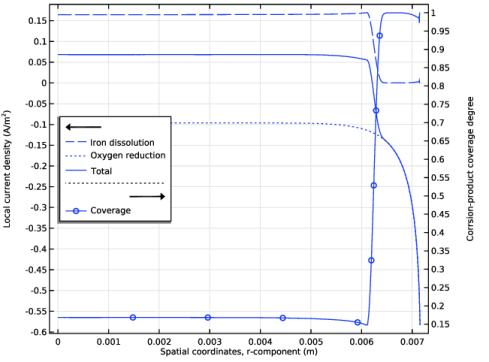
In the Settings window for 1D Plot Group, type Local Current Density and Coverage in the Label text field.
3
Click to expand the Title section. From the Title type list, choose None.
4
Locate the Data section. From the Time selection list, choose Last.
5
Locate the Plot Settings section. Select the Two y-axes checkbox.
6
Locate the Legend section. From the Position list, choose Middle left.
7
Locate the Plot Settings section.
8
Select the y-axis label checkbox. In the associated text field, type Local current density (A/m<sup>2</sup>).
9
Select the Secondary y-axis label checkbox. In the associated text field, type Corrosion-product coverage degree.
10
Select the x-axis label checkbox. In the associated text field, type Spatial coordinates, r-component (m).
Line Graph 1
1
Right-click Local Current Density and Coverage and choose Line Graph.
2
3
In the Settings window for Line Graph, locate the y-Axis Data section.
4
In the Expression text field, type aqt.es1.er1.iloc.
5
Locate the x-Axis Data section. From the Parameter list, choose Expression.
6
In the Expression text field, type r.
7
Click to expand the Coloring and Style section. Find the Line style subsection. From the Line list, choose Dashed.
8
Click to expand the Legends section. Select the Show legends checkbox.
9
From the Legends list, choose Manual.
10
Line Graph 2
1
In the Model Builder window, right-click Local Current Density and Coverage and choose Line Graph.
2
3
In the Settings window for Line Graph, locate the y-Axis Data section.
4
In the Expression text field, type aqt.es1.er2.iloc.
5
Locate the x-Axis Data section. From the Parameter list, choose Expression.
6
In the Expression text field, type r.
7
Locate the Coloring and Style section. Find the Line style subsection. From the Line list, choose Dotted.
8
From the Color list, choose Cycle (reset).
9
Locate the Legends section. Select the Show legends checkbox.
10
From the Legends list, choose Manual.
11
Line Graph 3
1
Right-click Local Current Density and Coverage and choose Line Graph.
2
3
In the Settings window for Line Graph, locate the y-Axis Data section.
4
In the Expression text field, type aqt.itot.
5
Locate the x-Axis Data section. From the Parameter list, choose Expression.
6
In the Expression text field, type r.
7
Locate the Coloring and Style section. From the Color list, choose Cycle (reset).
8
Locate the Legends section. Select the Show legends checkbox.
9
From the Legends list, choose Manual.
10
Line Graph 4
1
Right-click Local Current Density and Coverage and choose Line Graph.
2
3
In the Settings window for Line Graph, locate the y-Axis Data section.
4
In the Expression text field, type theta.
5
Locate the x-Axis Data section. From the Parameter list, choose Expression.
6
In the Expression text field, type r.
7
Locate the Coloring and Style section. From the Color list, choose Cycle (reset).
8
Find the Line markers subsection. From the Marker list, choose Circle.
9
From the Positioning list, choose Interpolated.
10
Locate the Legends section. Select the Show legends checkbox.
11
From the Legends list, choose Manual.
12
Local Current Density and Coverage
1
In the Model Builder window, click Local Current Density and Coverage.
2
In the Settings window for 1D Plot Group, locate the Plot Settings section.
3
In the table, select the Plot on secondary y-axis checkbox for Line Graph 4.
4
In the Local Current Density and Coverage toolbar, click  Plot.
Concentration, Fe, 3D
1
In the Results toolbar, click  3D Plot Group.
Finish with two 3D plots of the local Fe and CO2 concentration.
2
In the Settings window for 3D Plot Group, locate the Data section.
3
From the Dataset list, choose Revolution 2D 2.
4
In the Label text field, type Concentration, Fe, 3D.
Surface 1
1
Right-click Concentration, Fe, 3D and choose Surface.
2
In the Settings window for Surface, locate the Expression section.
3
In the Expression text field, type aqt.c3_Fe.
4
In the Concentration, Fe, 3D toolbar, click  Plot.
Concentration, Fe, 3D
1
In the Model Builder window, click Concentration, Fe, 3D.
2
In the Settings window for 3D Plot Group, locate the Data section.
3
From the Time (s) list, choose 10.
4
In the Concentration, Fe, 3D toolbar, click  Plot.
5
From the Time (s) list, choose 300.
6
In the Concentration, Fe, 3D toolbar, click  Plot.
Concentration, CO2, 3D
1
In the Results toolbar, click  3D Plot Group.
2
In the Settings window for 3D Plot Group, locate the Data section.
3
From the Dataset list, choose Revolution 2D 2.
4
In the Label text field, type Concentration, CO2, 3D.
Surface 1
1
Right-click Concentration, CO2, 3D and choose Surface.
2
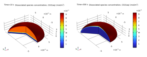
In the Settings window for Surface, click Replace Expression in the upper-right corner of the Expression section. From the menu, choose Component 1 (comp1) > Aqueous Electrolyte Transport > Carbonic Acid 1 > aqt.c4_H2CO3 - Dissociated species concentration, CO2(aq) - mol/m³.
3
In the Concentration, CO2, 3D toolbar, click  Plot.
Concentration, CO2, 3D
1
In the Model Builder window, click Concentration, CO2, 3D.
2
In the Settings window for 3D Plot Group, locate the Data section.
3
From the Time (s) list, choose 10.
4
In the Concentration, CO2, 3D toolbar, click  Plot.
5
From the Time (s) list, choose 300.
6
In the Concentration, CO2, 3D toolbar, click  Plot.