|
|
|
|
Fe2+
|
|
|
FeOH+
|
|
|
Na+
|
|


|
1
|
|
2
|
|
3
|
Click Add.
|
|
4
|
Click
|
|
5
|
|
6
|
Click
|
|
1
|
|
2
|
|
3
|
Click
|
|
4
|
Browse to the model’s Application Libraries folder and double-click the file crevice_corrosion_fe_parameters.txt.
|
|
1
|
|
2
|
|
4
|
Click
|
|
5
|
|
1
|
|
2
|
Go to the Add Material window.
|
|
3
|
|
4
|
Click the Add to Component button in the window toolbar.
|
|
5
|
|
1
|
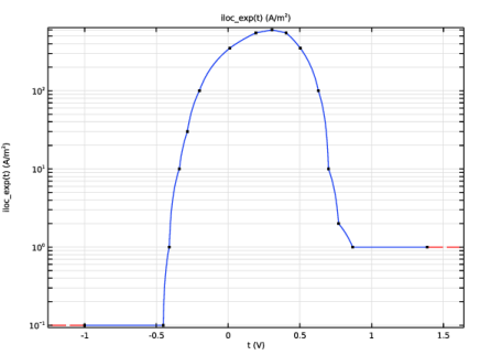
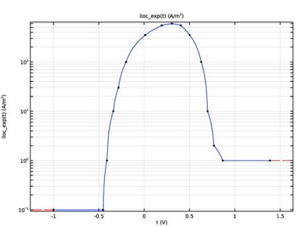
In the Model Builder window, expand the Component 1 (comp1) > Materials > Fe in acetic acid/sodium acetate (Anodic) (mat1) > Local current density (lcd) node, then click Interpolation 1 (iloc_exp).
|
|
2
|
|
3
|
|
1
|
In the Model Builder window, under Component 1 (comp1) > Aqueous Electrolyte Transport (aqt) click Electrolyte 1.
|
|
2
|
|
3
|
|
1
|
|
2
|
In the Settings window for Fully Dissociated Species, type Fully Dissociated Species - Fe in the Label text field.
|
|
3
|
|
4
|
|
5
|
|
1
|
In the Settings window for Fully Dissociated Species, type Fully Dissociated Species - Na in the Label text field.
|
|
2
|
|
3
|
|
4
|
|
1
|
|
2
|
|
3
|
|
4
|
|
1
|
|
2
|
|
3
|
|
4
|
|
5
|
|
6
|
Select the OH checkbox.
|
|
7
|
|
8
|
|
1
|
|
2
|
In the Settings window for Complex Species, type Complex Species - CH3COOFe in the Label text field.
|
|
3
|
|
4
|
|
5
|
|
6
|
Select the CH3COOH (-1) checkbox.
|
|
7
|
|
8
|
|
1
|
In the Model Builder window, under Component 1 (comp1) > Aqueous Electrolyte Transport (aqt) click Initial Values 1.
|
|
2
|
|
3
|
|
4
|
|
5
|
|
6
|
|
1
|
|
2
|
|
3
|
|
4
|
|
5
|
|
1
|
In the Model Builder window, expand the Highly Conductive Porous Electrode 1 node, then click Porous Electrode Reaction 1.
|
|
2
|
|
3
|
|
4
|
|
5
|
|
6
|
|
1
|
|
3
|
|
4
|
|
5
|
|
6
|
|
7
|
|
8
|
|
1
|
In the Model Builder window, under Component 1 (comp1) right-click Mesh 1 and choose Edit Physics-Induced Sequence.
|
|
1
|
|
2
|
|
3
|
Click the Custom button.
|
|
4
|
|
5
|
|
1
|
|
2
|
|
3
|
|
5
|
|
6
|
Locate the Element Size Parameters section.
|
|
7
|
|
1
|
|
2
|
|
3
|
Select the Auxiliary sweep checkbox.
|
|
4
|
Click
|
|
6
|
|
7
|
|
8
|
Clear the Generate default plots checkbox.
|
|
9
|
|
1
|
|
2
|
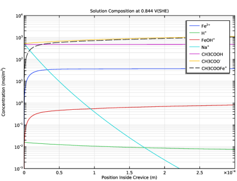
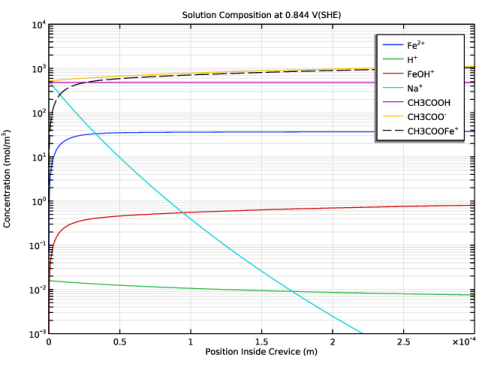
In the Settings window for 1D Plot Group, type Solution Composition at 0.844 V(SHE) in the Label text field.
|
|
3
|
|
4
|
|
5
|
Locate the Plot Settings section.
|
|
6
|
|
7
|
Select the y-axis label checkbox. In the associated text field, type Concentration (mol/m<sup>3</sup>).
|
|
1
|
|
2
|
|
3
|
|
4
|
Click Replace Expression in the upper-right corner of the y-Axis Data section. From the menu, choose Component 1 (comp1) > Aqueous Electrolyte Transport > Fully Dissociated Species - Fe > aqt.c_Fe - Concentration, Fe species - mol/m³.
|
|
5
|
|
6
|
|
1
|
|
2
|
In the Settings window for Line Graph, click Replace Expression in the upper-right corner of the y-Axis Data section. From the menu, choose Component 1 (comp1) > Aqueous Electrolyte Transport > Electrolyte 1 > aqt.cH - Proton concentration - mol/m³.
|
|
3
|
Locate the Legends section. In the table, enter the following settings:
|
|
1
|
|
2
|
In the Settings window for Line Graph, click Replace Expression in the upper-right corner of the y-Axis Data section. From the menu, choose Component 1 (comp1) > Aqueous Electrolyte Transport > Complex Species - FeOH > aqt.el1.coms1.c_comp - Complex species concentration - mol/m³.
|
|
3
|
Locate the Legends section. In the table, enter the following settings:
|
|
1
|
|
2
|
In the Settings window for Line Graph, click Replace Expression in the upper-right corner of the y-Axis Data section. From the menu, choose Component 1 (comp1) > Aqueous Electrolyte Transport > Fully Dissociated Species - Na > aqt.c_Na - Concentration, Na species - mol/m³.
|
|
3
|
Locate the Legends section. In the table, enter the following settings:
|
|
1
|
|
2
|
In the Settings window for Line Graph, click Replace Expression in the upper-right corner of the y-Axis Data section. From the menu, choose Component 1 (comp1) > Aqueous Electrolyte Transport > Weak Acid - CH3COOH > Dissociated species concentrations - mol/m³ > aqt.c2_CH3COOH - Concentration, species with 0 charge.
|
|
3
|
Locate the Legends section. In the table, enter the following settings:
|
|
1
|
|
2
|
In the Settings window for Line Graph, click Replace Expression in the upper-right corner of the y-Axis Data section. From the menu, choose Component 1 (comp1) > Aqueous Electrolyte Transport > Weak Acid - CH3COOH > Dissociated species concentrations - mol/m³ > aqt.c1_CH3COOH - Concentration, species with -1 charge.
|
|
3
|
Locate the Legends section. In the table, enter the following settings:
|
|
1
|
|
2
|
In the Settings window for Line Graph, click Replace Expression in the upper-right corner of the y-Axis Data section. From the menu, choose Component 1 (comp1) > Aqueous Electrolyte Transport > Complex Species - CH3COOFe > aqt.el1.coms2.c_comp - Complex species concentration - mol/m³.
|
|
3
|
Locate the Legends section. In the table, enter the following settings:
|
|
4
|
Click to expand the Coloring and Style section. Find the Line style subsection. From the Line list, choose Dashed.
|
|
1
|
|
2
|
|
3
|
Select the y-axis log scale checkbox.
|
|
4
|
Select the Manual axis limits checkbox.
|
|
5
|
|
6
|
|
7
|
|
8
|
|
9
|
|
1
|
|
2
|
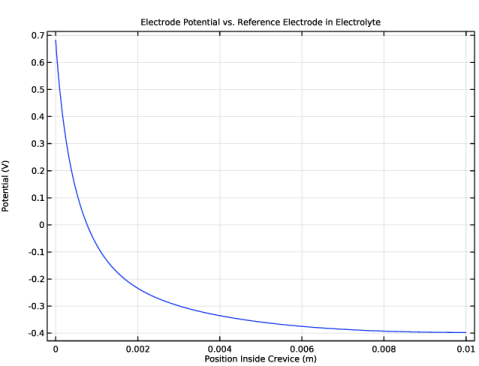
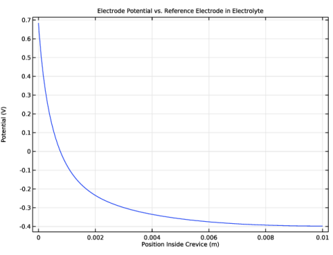
In the Settings window for 1D Plot Group, type Electrode Potential vs. Reference Electrode in Electrolyte in the Label text field.
|
|
3
|
|
4
|
|
5
|
Locate the Plot Settings section.
|
|
6
|
|
7
|
|
1
|
|
3
|
|
4
|
|
5
|
|
1
|
|
2
|
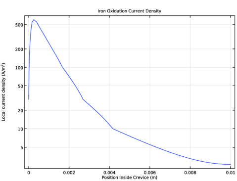
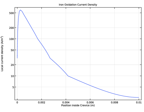
In the Settings window for 1D Plot Group, type Iron Oxidation Current Density in the Label text field.
|
|
3
|
|
4
|
|
5
|
|
1
|
|
3
|
In the Settings window for Line Graph, click Replace Expression in the upper-right corner of the y-Axis Data section. From the menu, choose Component 1 (comp1) > Aqueous Electrolyte Transport > Electrode kinetics > aqt.hcpce1.per1.iloc - Local current density - A/m².
|
|
4
|
|
5
|
Click Replace Expression in the upper-right corner of the x-Axis Data section. From the menu, choose Component 1 (comp1) > Geometry > Coordinate > x - x-coordinate.
|
|
6
|
Locate the x-Axis Data section.
|
|
7
|
|
8
|