PDF

Estimation of Corrosion Kinetics Parameters
Introduction
A common challenge in corrosion modeling is to accurately describe the electrode kinetics as a function of electrode potential. This tutorial shows how to use the Parameter Estimation study node to perform electrode kinetics parameter estimations based on polarization data.
A zero-dimensional electrode polarization model is constructed using an anode Tafel expression for the metal dissolution reaction and a cathode Tafel expression for the oxygen reduction kinetics in combination with an oxygen reduction limiting current density.
Parameter estimation is performed using a global least-squares objective function based on three different sets of polarization data (Ref. 1) recorded for the following metals:
The experimental data was recorded using potentiodynamic scans at 30°C for fresh metals in a controlled sea water flow (8.0 ft/s) environment.
Model Definition
The metal dissolution reaction is described by an anodic Tafel expression according to:
(1)
where i0, Me (A/m2) is the exchange current density and AMe (V) is the anodic Tafel slope of the metal dissolution reaction, respectively. The overpotential of the metal dissolution reaction, ηMe (V), is defined as:
(2)
where Eeq, Me is the equilibrium potential of the metal dissolution reaction. Note that the choice of Eeq, Me (which is generally unknown) is arbitrary in this model since the cathodic part of the metal dissolution reaction is neglected. Eeq,Me = 0 is used in this model.
For the oxygen reduction reaction, the following cathodic Tafel expression is used:
(3)
where i0,O2 (A/m2) is the exchange current density and AO2 (V) is the cathodic Tafel slope of the oxygen reduction reaction, respectively. The overpotential of the oxygen reduction reaction, ηO2 (V), is defined as:
(4)
The equilibrium potential for oxygen reduction is defined to be dependent on the pH according to the Nernst equation:
(5)
where T (K) is the temperature. (But note that here also the actual choice of Eeq,O2 is arbitrary). A pH of 7.7 is used in the model.
Furthermore, the current density of oxygen is assumed to be limited by diffusion, resulting in:
(6)
where iO2,lim (A/m2) is the limiting current density for oxygen reduction.
Finally, the total current density at the electrode surface, iloc (A/m2), is:
(7)
Note that for low potentials one should also consider hydrogen evolution as an additional cathodic reaction. That reaction is however not included in this tutorial.
The model is formulated as a set of parametric expressions in 0D and the Parameter Estimation study node is used to create a least squares objective function used for optimization, based on the experimental data.
Results and Discussion
The experimental polarization curves for the 70-30 Cu-Ni alloy and the corresponding fitted model values are shown in Figure 1 and Figure 2, using a linear or a logarithmic scale for the current density values, respectively.
Figure 3 and Figure 4 show the polarization curves in logarithmic scale for the 90-10 Cu-Ni and the Ni-Al bronze. In all cases, the model seems to be able to capture the salient features of the polarization behavior.
Table 1 shows the fitted parameter values for the polarization data for the three different metals. The two Cu-Ni alloys exhibit fairly similar values, whereas the values for the Ni-Al bronze are more different. The limiting current density for oxygen reduction are similar for all cases. This is expected since the experiments where conducted for fresh metals in a controlled flow environment.
AMe
AO2
i0,Me
103.3
102.8
103.5
i0,O2
10-7.1
10-7.3
10-10
iO2,lim
Figure 1: Polarization curve (linear scale) for the 70-30 Cu-Ni alloy.
Figure 2: Polarization curve (log scale) for the 70-30 Cu-Ni alloy.
Figure 3: Polarization curve (log scale) for the 90-10 Cu-Ni alloy.
Figure 4: Polarization curve (log scale) for the Ni-Al bronze.
Reference
1. Atlas of Polarization Diagrams for Naval Materials in Seawater. Harvey P Hack. Carderock Division, Naval Surface Warfare Center, CARDIVNSWC-TR-61 -94/44, April 1995.
Application Library path: Corrosion_Module/General_Corrosion/corrosion_parameter_estimation
Modeling Instructions
From the File menu, choose New.
New
In the New window, click  Blank Model.
Add Component
In the Home toolbar, click  Add Component and choose 0D.
Global Definitions
Load the model parameters from a text file.
Parameters 1
1
In the Model Builder window, under Global Definitions click Parameters 1.
2
In the Settings window for Parameters, locate the Parameters section.
3
Click  Load from File.
4
Definitions
Interpolation 1 (int1)
1
In the Definitions toolbar, click  Interpolation.
2
In the Settings window for Interpolation, locate the Definition section.
3
From the Data source list, choose File.
4
In the Filename text field, type 7030CuNi_pol.csv.
5
Click  Import.
Interpolation 2 (int2)
1
Right-click Interpolation 1 (int1) and choose Duplicate.
2
In the Settings window for Interpolation, locate the Definition section.
3
From the Data source list, choose File.
4
In the Filename text field, type 9010CuNi_pol.csv.
5
Click  Import.
Interpolation 3 (int3)
1
Right-click Interpolation 2 (int2) and choose Duplicate.
2
In the Settings window for Interpolation, locate the Definition section.
3
From the Data source list, choose File.
4
In the Filename text field, type NiAlBronze_pol.csv.
5
Click  Import.
Add Study
1
In the Home toolbar, click  Add Study to open the Add Study window.
2
Go to the Add Study window.
3
Find the Studies subsection. In the Select Study tree, select Preset Studies for Selected Physics Interfaces > Stationary.
4
Click the Add Study button in the window toolbar three times.
5
In the Study toolbar, click  Add Study to close the Add Study window.
Study 1
Use the Parameter Estimation study step to specify the polarization data (70-30 Cu-Ni) used by the optimization solver. The objective function will be created automatically by the study step.
Parameter Estimation
1
In the Study toolbar, click  Optimization and choose Parameter Estimation.
2
In the Settings window for Parameter Estimation, locate the Experimental Data section.
3
In the Filename text field, type 7030CuNi_pol.csv.
4
Click  Refresh.
5
Locate the Data Column Settings section. In the table, click to select the cell at row number 1 and column number 2.
6
7
From the Name list, choose E (Electrode potential).
8
In the text fields that appear below the table, enter the following values:
9
In the Model expression text field, type iloc.
10
In the Column name text field, type iloc_exp.
11
In the Unit text field, type A/m^2.
12
From the Scale list, choose Manual.
13
In the Scale value text field, type max(abs(comp1.int1(E)),1e-2).
14
Locate the Estimated Parameters section. Click  Add five times.
15
Since there is no need to constrain the optimization parameters (control variables) for this least-squares problem, the Levenberg–Marquardt method is suitable.
16
Locate the Parameter Estimation Method section. From the Method list, choose Levenberg–Marquardt.
17
From the Least-squares time/parameter list method list, choose Merge within manual range.
18
In the Optimality tolerance text field, type 1e-4.
Component 1 (comp1)
By adding global probes for the optimization parameters, one can monitor the progress of the optimization during the computation.
Definitions
Global Variable Probe 1 (var1)
1
In the Definitions toolbar, click  Probes and choose Global Variable Probe.
2
In the Settings window for Global Variable Probe, locate the Expression section.
3
In the Expression text field, type A_O2.
Global Variable Probe 2 (var2)
1
In the Definitions toolbar, click  Probes and choose Global Variable Probe.
2
In the Settings window for Global Variable Probe, locate the Expression section.
3
In the Expression text field, type A_Me.
Global Variable Probe 3 (var3)
1
In the Definitions toolbar, click  Probes and choose Global Variable Probe.
2
In the Settings window for Global Variable Probe, locate the Expression section.
3
In the Expression text field, type log10_i0_O2.
Global Variable Probe 4 (var4)
1
In the Definitions toolbar, click  Probes and choose Global Variable Probe.
2
In the Settings window for Global Variable Probe, locate the Expression section.
3
In the Expression text field, type log10_i0_Me.
Global Variable Probe 5 (var5)
1
In the Definitions toolbar, click  Probes and choose Global Variable Probe.
2
In the Settings window for Global Variable Probe, locate the Expression section.
3
In the Expression text field, type i_O2_lim.
70-30 Cu-Ni
1
In the Model Builder window, click Study 1.
2
In the Settings window for Study, type 70-30 Cu-Ni in the Label text field.
The model is now ready for solving.
3
Locate the Study Settings section. Clear the Generate default plots checkbox.
4
In the Study toolbar, click  Compute.
The last row of the probe table now shows the final values of the optimization parameters.
Results
Create polarization plots as follows:
1D Plot Group 2
In the Results toolbar, click  1D Plot Group.
Global 1
1
Right-click 1D Plot Group 2 and choose Global.
2
In the Settings window for Global, locate the y-Axis Data section.
3
4
Locate the x-Axis Data section. From the Parameter list, choose Expression.
5
In the Expression text field, type comp1.int1(E).
6
Click to expand the Coloring and Style section. Find the Line style subsection. From the Line list, choose None.
7
Find the Line markers subsection. From the Marker list, choose Cycle.
8
Click to expand the Legends section. From the Legends list, choose Manual.
9
Global 2
1
In the Model Builder window, right-click 1D Plot Group 2 and choose Global.
2
In the Settings window for Global, locate the y-Axis Data section.
3
4
Locate the x-Axis Data section. From the Parameter list, choose Expression.
5
In the Expression text field, type iloc.
6
Locate the Legends section. From the Legends list, choose Manual.
7
8
In the 1D Plot Group 2 toolbar, click  Plot.
Global 3
1
Right-click Global 2 and choose Duplicate.
2
In the Settings window for Global, locate the x-Axis Data section.
3
In the Expression text field, type i_Me.
4
Locate the Legends section. In the table, enter the following settings:
5
In the 1D Plot Group 2 toolbar, click  Plot.
Global 4
1
Right-click Global 3 and choose Duplicate.
2
In the Settings window for Global, locate the x-Axis Data section.
3
In the Expression text field, type i_O2.
4
Locate the Legends section. In the table, enter the following settings:
Polarization plot 70-30 Cu-Ni (linear scale)
1
In the Model Builder window, under Results click 1D Plot Group 2.
2
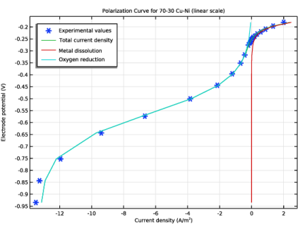
In the Settings window for 1D Plot Group, type Polarization plot 70-30 Cu-Ni (linear scale) in the Label text field.
3
Click to expand the Title section. From the Title type list, choose Manual.
4
In the Title text area, type Polarization Curve for 70-30 Cu-Ni (linear scale).
5
Locate the Plot Settings section.
6
Select the x-axis label checkbox. In the associated text field, type Current density (A/m<sup>2</sup>).
7
Locate the Legend section. From the Position list, choose Upper left.
8
In the Polarization plot 70-30 Cu-Ni (linear scale) toolbar, click  Plot.
Polarization plot 70-30 Cu-Ni (log scale)
1
Right-click Polarization plot 70-30 Cu-Ni (linear scale) and choose Duplicate.
2
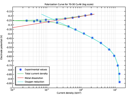
In the Settings window for 1D Plot Group, type Polarization plot 70-30 Cu-Ni (log scale) in the Label text field.
3
Locate the Title section. In the Title text area, type Polarization Curve for 70-30 Cu-Ni (log scale).
4
Click the  x-Axis Log Scale button in the Graphics toolbar.
Global 1
For the log plot, only positive current densities can be plotted.
1
In the Model Builder window, expand the Polarization plot 70-30 Cu-Ni (log scale) node, then click Global 1.
2
In the Settings window for Global, locate the x-Axis Data section.
3
In the Expression text field, type abs(comp1.int1(E)).
Global 2
1
In the Model Builder window, click Global 2.
2
In the Settings window for Global, locate the x-Axis Data section.
3
In the Expression text field, type abs(iloc).
Global 3
The metal dissolution currents are always positive, so there is no need to modify this expression.
Global 4
1
In the Model Builder window, click Global 4.
2
In the Settings window for Global, locate the x-Axis Data section.
3
In the Expression text field, type abs(i_O2).
4
In the Polarization plot 70-30 Cu-Ni (log scale) toolbar, click  Plot.
Polarization plot 70-30 Cu-Ni (log scale)
1
In the Model Builder window, click Polarization plot 70-30 Cu-Ni (log scale).
2
In the Settings window for 1D Plot Group, locate the Axis section.
3
Select the Manual axis limits checkbox.
4
In the x minimum text field, type 1e-2.
5
In the x maximum text field, type 20.
6
In the y minimum text field, type -1.
7
In the y maximum text field, type -0.1.
8
In the Polarization plot 70-30 Cu-Ni (log scale) toolbar, click  Plot.
9
Locate the Legend section. From the Position list, choose Lower left.
10
In the Polarization plot 70-30 Cu-Ni (log scale) toolbar, click  Plot.
Now perform the same optimization for a different dataset (90-10 Cu-Ni).
70-30 Cu-Ni
Parameter Estimation
In the Model Builder window, under 70-30 Cu-Ni right-click Parameter Estimation and choose Copy.
90-10 Cu-Ni
In the Model Builder window, right-click Study 2 and choose Paste Parameter Estimation.
1
In the Settings window for Parameter Estimation, locate the Experimental Data section.
2
In the Filename text field, type 9010CuNi_pol.csv.
3
Click  Refresh.
4
Locate the Data Column Settings section. In the table, click to select the cell at row number 2 and column number 3.
5
6
From the Scale list, choose Manual.
7
In the Scale value text field, type max(abs(comp1.int2(E)),1e-2).
8
In the Model Builder window, click Study 2.
9
In the Settings window for Study, type 90-10 Cu-Ni in the Label text field.
10
Locate the Study Settings section. Clear the Generate default plots checkbox.
11
In the Study toolbar, click  Compute.
Results
Polarization plot 90-10 Cu-Ni (linear scale)
1
In the Model Builder window, right-click Polarization plot 70-30 Cu-Ni (linear scale) and choose Duplicate.
2
In the Settings window for 1D Plot Group, type Polarization plot 90-10 Cu-Ni (linear scale) in the Label text field.
3
Locate the Data section. From the Dataset list, choose 90-10 Cu-Ni/Solution 2 (sol2).
4
Locate the Title section. In the Title text area, type Polarization Curve for 90-10 Cu-Ni (linear scale).
Global 1
1
In the Model Builder window, expand the Polarization plot 90-10 Cu-Ni (linear scale) node, then click Global 1.
2
In the Settings window for Global, locate the x-Axis Data section.
3
In the Expression text field, type comp1.int2(E).
Polarization plot 90-10 Cu-Ni (log scale)
1
In the Model Builder window, right-click Polarization plot 70-30 Cu-Ni (log scale) and choose Duplicate.
2
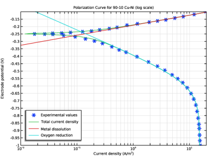
In the Settings window for 1D Plot Group, type Polarization plot 90-10 Cu-Ni (log scale) in the Label text field.
3
Locate the Data section. From the Dataset list, choose 90-10 Cu-Ni/Solution 2 (sol2).
4
Locate the Title section. In the Title text area, type Polarization Curve for 90-10 Cu-Ni (log scale).
Global 1
1
In the Model Builder window, expand the Polarization plot 90-10 Cu-Ni (log scale) node, then click Global 1.
2
In the Settings window for Global, locate the x-Axis Data section.
3
In the Expression text field, type abs(comp1.int2(E)).
4
In the Polarization plot 90-10 Cu-Ni (log scale) toolbar, click  Plot.
Finally, also try the optimization on a polarization for a Ni-Al bronze.
70-30 Cu-Ni
Parameter Estimation
In the Model Builder window, under 70-30 Cu-Ni right-click Parameter Estimation and choose Copy.
Ni-Al Bronze
In the Model Builder window, right-click Study 3 and choose Paste Parameter Estimation.
1
In the Settings window for Parameter Estimation, locate the Experimental Data section.
2
In the Filename text field, type NiAlBronze_pol.csv.
3
Click  Refresh.
4
Locate the Data Column Settings section. In the table, click to select the cell at row number 2 and column number 3.
5
6
From the Scale list, choose Manual.
7
In the Scale value text field, type max(abs(comp1.int3(E)),1e-2).
8
In the Model Builder window, click Study 3.
9
In the Settings window for Study, type Ni-Al Bronze in the Label text field.
10
Locate the Study Settings section. Clear the Generate default plots checkbox.
11
In the Study toolbar, click  Compute.
Results
Polarization plot Ni-Al (linear scale)
1
In the Model Builder window, right-click Polarization plot 70-30 Cu-Ni (linear scale) and choose Duplicate.
2
In the Settings window for 1D Plot Group, type Polarization plot Ni-Al (linear scale) in the Label text field.
3
Locate the Data section. From the Dataset list, choose Ni-Al Bronze/Solution 3 (sol3).
4
Locate the Title section. In the Title text area, type Polarization Curve for Ni-Al Bronze (linear scale).
Global 1
1
In the Model Builder window, expand the Polarization plot Ni-Al (linear scale) node, then click Global 1.
2
In the Settings window for Global, locate the x-Axis Data section.
3
In the Expression text field, type comp1.int3(E).
Polarization plot Ni-Al (log scale)
1
In the Model Builder window, right-click Polarization plot 70-30 Cu-Ni (log scale) and choose Duplicate.
2
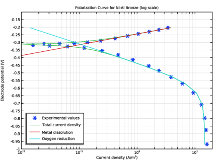
In the Settings window for 1D Plot Group, type Polarization plot Ni-Al (log scale) in the Label text field.
3
Locate the Data section. From the Dataset list, choose Ni-Al Bronze/Solution 3 (sol3).
4
Locate the Title section. In the Title text area, type Polarization Curve for Ni-Al Bronze (log scale).
Global 1
1
In the Model Builder window, expand the Polarization plot Ni-Al (log scale) node, then click Global 1.
2
In the Settings window for Global, locate the x-Axis Data section.
3
In the Expression text field, type abs(comp1.int3(E)).
4
In the Polarization plot Ni-Al (log scale) toolbar, click  Plot.