PDF

Carbon Dioxide Corrosion in Steel Pipes
Introduction
A flow mixture of water and carbon dioxide (CO2) passing through a steel pipe can cause significant steel corrosion. Properties such as partial pressure of CO2 and temperature affect the corrosion rate.
This model simulates the corrosion taking place on the steel surface of a pipe carrying CO2 and water mixture. The model is based on several journal papers (Ref. 1Ref. 4).
Model Definition
The corrosion is investigated at an arbitrary position within a steel pipe through which a flow of dissolved CO2 in water passes. A 1D model is used. No variations along the length of the pipe are considered and the interaction of the mixture with the steel is confined to the boundary layer near the steel surface. The boundary layer thickness is considered to be 50 μm. The model geometry is shown in Figure 1.
Figure 1: The model geometry comprising of the boundary layer adjacent to the steel surface.
All species are assumed to be diluted in water and the mass transport is modeled by diffusion and migration. The Aqueous Electrolyte Transport interface is used in the model. Water dissociation, carbonic acid dissociation, and ferrous ion hydrolysis are accounted for; resulting in eight species in the model. The species and diffusion coefficients are tabulated in Table 1.
D (m2/s)·10-9
CO2(aq)
H2CO3
HCO3-
CO32-
H+
Fe2+, FeOH+, Fe(OH)2(aq)
The Electrode Surface boundary feature is used to calculate the corrosion potential at the steel surface. The electric potential is set to 0 at the steel surface which will result in a mixed potential condition since the electrolyte potential is left to float. The initial value of the electrolyte potential is set to 0.5 V, close to the free corrosion potential (Ref. 3).
Fluxes of species, Ji (mol/m2·s), converted in the electrochemical reactions are applied on the steel surface in accordance to Faraday’s law
where νi is the stoichiometric coefficient for reactant i, ij,loc (A/m2) the current density for reaction j, n the number of transferred electrons, and F Faraday’s constant (96,485 As/mol)
Uniform total concentrations of carbonic acid species and ferrous species are used as initial values for the concentration.
Equilibrium Reactions
These are the equilibrium reactions present in the electrolyte:
where K1 through K6 are the equilibrium constants at 298.15 K (Ref. 1 and Ref. 2).
The water dissociation equilibrium reaction is built in for the interface. The carbonic acid can be added with the Carbonic Acid node that is customized for these reactions. The ferrous ion hydrolysis reactions are defined using the Ampholyte node.
Electrochemical Reactions
The following electrochemical reactions are present at the steel surface:
Study Settings
The problem is solved with an auxiliary sweep on a stationary solver in order to investigate the impact of important parameters such as partial pressure of CO2 and temperature on corrosion.
Results and Discussion
Figure 2 displays the concentration deviation from the bulk of the four species along the boundary layer at partial pressure of CO2 of 1 bar and 20ºC. The concentration of iron ions is significantly higher at the steel surface due to the dissolution of iron. The deviation between carbon dioxide and bicarbonate ions show considerable dissociation of the carbon dioxide.
Figure 2: Deviation in concentration of the species compared to the bulk along the liquid boundary layer.
Figure 3 shows the corrosion rate of the steel surface at different partial pressures of CO2 for operating temperatures ranging from 20ºC to 80ºC. The corrosion rate is directly proportional to the corrosion current (that is, the iron dissolution current, since no other anodic reaction is considered). Increased partial pressure of CO2 and temperature increase the corrosion rate.
Figure 3: Corrosion rate in mm/year for different partial pressures of CO2 and operating temperatures in the range 20ºC–80ºC.
Figure 4 and Figure 5 show the change in pH at the steel surface and bulk electrolyte, respectively, for different partial pressures of CO2 and for operating temperatures ranging from 20ºC to 80ºC. The higher pH is observed for lower partial pressure of CO2 at both the electrode surface as well as the bulk electrolyte for all operating temperatures considered in the model. The increase in pH with an increase in temperature is observed to be more significant at the electrode surface when compared to the bulk electrolyte.
Figure 4: pH at the electrode surface for different partial pressures of CO2 and operating temperatures in the range 20ºC–80ºC.
Figure 5: pH at the bulk electrolyte for different partial pressures of CO2 and operating temperatures in the range 20ºC–80ºC.
References
1. M. Nordsveen, S. Nesic, R. Nyborg, and A. Stangeland, “A Mechanistic Model for Carbon Dioxide Corrosion of Mild Steel in the Presence of Protective Iron Carbonate Films-Part 1: theory and Verification,” Corrosion, vol. 59, no. 5, pp. 443–455, 2003.
2. F. J. Millero, W. Yao, and J. Aicher, “The speciation of Fe(II) and Fe(III) in natural waters,” Marine Chemistry, vol. 50, pp. 21–39, 1995.
3. S. Nesic, J. Postlethwaite, and S. Olsen, “An Electrochemical Model for Prediction of Corrosion of Mild Steel in Aqueous Carbon Dioxide Solutions,” Corrosion, vol. 52, no. 4, pp. 280–294, 1996.
4. A. Kahyarian and S. Nesic, “On the mechanism of carbon dioxide corrosion of mild steel: Experimental investigation and mathematical modeling at elevated pressures and non-ideal solutions,” Corrosion Science, vol. 173, no. 108719, pp. 1–27, 2020.
Application Library path: Corrosion_Module/General_Corrosion/co2_corrosion
Modeling Instructions
From the File menu, choose New.
New
In the New window, click  Model Wizard.
Model Wizard
1
In the Model Wizard window, click  1D.
2
In the Select Physics tree, select Electrochemistry > Aqueous Electrolyte Transport (aqt).
3
Click Add.
4
Click  Study.
5
In the Select Study tree, select General Studies > Stationary.
6
Global Definitions
Load the model parameters from a text file.
Parameters 1
1
In the Model Builder window, under Global Definitions click Parameters 1.
2
In the Settings window for Parameters, locate the Parameters section.
3
Click  Load from File.
4
Geometry 1
The geometry consists of a single interval.
Interval 1 (i1)
1
In the Model Builder window, under Component 1 (comp1) right-click Geometry 1 and choose Interval.
2
In the Settings window for Interval, locate the Interval section.
3
4
Click  Build Selected.
Aqueous Electrolyte Transport (aqt)
Define the physics, start with the solvent (water) parameters.
Electrolyte 1
1
In the Model Builder window, under Component 1 (comp1) > Aqueous Electrolyte Transport (aqt) click Electrolyte 1.
2
In the Settings window for Electrolyte, locate the Proton and Hydroxide Ion Transport Properties section.
3
In the DH+ text field, type DH.
4
In the DOH text field, type DOH.
Add an Ampholyte node and define the ferrous ion hydrolysis reactions.
5
In the Model Builder window, click Electrolyte 1.
Ampholyte - Fe
1
In the Physics toolbar, click  Attributes and choose Ampholyte.
2
In the Settings window for Ampholyte, type Ampholyte - Fe in the Label text field.
3
Locate the Ampholyte section. In the Species name text field, type Fe.
4
5
In the z0 text field, type 0.
6
Locate the Diffusion and Migration section. In the D text field, type DFe.
Add a Carbonic Acid node that is solely devoted to dissociated species of carbonic acid.
Electrolyte 1
In the Model Builder window, click Electrolyte 1.
Carbonic Acid 1
In the Physics toolbar, click  Attributes and choose Carbonic Acid.
Set the initial values. The interface computes all hydrolyzed (Ampholyte - Fe) and dissociated (Carbonic Acid) species (that is, the species originating from the equilibrium reactions) automatically. Only the total species concentrations are required to be set. For the carbonic acid, the solution is assumed to be saturated with aqueous carbon dioxide.
Initial Values 1
1
In the Model Builder window, under Component 1 (comp1) > Aqueous Electrolyte Transport (aqt) click Initial Values 1.
2
In the Settings window for Initial Values, locate the Electrolyte Potential section.
3
In the ϕl,0 text field, type phil_init.
4
Locate the Concentration section. In the cH2CO3,0 text field, type cH2CO3_init.
Define the concentrations at the bulk boundary of the layer using the Reservoir node. Just as for the Initial Values settings, only total species concentrations are required.
Reservoir 1
1
In the Physics toolbar, click  Boundaries and choose Reservoir.
2
The reservoir is assumed to be completely saturated with aqueous carbon dioxide.
3
In the Settings window for Reservoir, locate the Concentration section.
4
In the c0,H2CO3 text field, type cH2CO30.
Define the electrochemical reactions with an Electrode Surface node.
Electrode Surface 1
1
In the Physics toolbar, click  Boundaries and choose Electrode Surface.
2
Use the Dissolving-Depositing species formulation to estimate the corrosion rate. Also, set fluxes according to the electrochemical reactions at the steel surface.
3
In the Settings window for Electrode Surface, click to expand the Dissolving–Depositing Species section.
4
5
Define each electrochemical reaction in an Electrode Reaction child node.
Electrode Reaction 1
1
In the Model Builder window, click Electrode Reaction 1.
2
In the Settings window for Electrode Reaction, locate the Stoichiometric Coefficients section.
3
In the νFe2+ text field, type -1.
4
Find the Stoichiometric coefficients for dissolving–depositing species subsection. In the table, enter the following settings:
5
Locate the Equilibrium Potential section. In the Eeq,ref(T) text field, type Eeq_ref_Fe.
6
Locate the Electrode Kinetics section. In the i0,ref(T) text field, type i0_ref_Fe.
7
In the αa text field, type alphaa_Fe.
Electrode Surface 1
In the Model Builder window, click Electrode Surface 1.
Electrode Reaction 2
1
In the Physics toolbar, click  Attributes and choose Electrode Reaction.
2
In the Settings window for Electrode Reaction, locate the Stoichiometric Coefficients section.
3
In the νH+ text field, type -1.
4
Locate the Equilibrium Potential section. In the Eeq,ref(T) text field, type Eeq_ref_H2.
5
Locate the Electrode Kinetics section. In the i0,ref(T) text field, type i0_ref_H2.
6
In the αa text field, type alphaa_H2.
Set up an integration operator for the bulk boundary for easier post processing.
Definitions
Bulk Boundary
1
In the Definitions toolbar, click  Nonlocal Couplings and choose Integration.
2
In the Settings window for Integration, type Bulk Boundary in the Label text field.
3
In the Operator name text field, type intop_bulk.
4
Locate the Source Selection section. From the Geometric entity level list, choose Boundary.
5
Mesh 1
Build a user-defined mesh with a maximum element size in the domain of 1e-6 and at the leftmost boundary 1e-7.
1
In the Model Builder window, under Component 1 (comp1) click Mesh 1.
2
In the Settings window for Mesh, locate the Sequence Type section.
3
From the list, choose User-controlled mesh.
Size
1
In the Model Builder window, under Component 1 (comp1) > Mesh 1 click Size.
2
In the Settings window for Size, locate the Element Size section.
3
Click the Custom button.
4
Locate the Element Size Parameters section. In the Maximum element size text field, type 1e-6.
Size 1
1
In the Model Builder window, right-click Edge 1 and choose Size.
2
In the Settings window for Size, locate the Geometric Entity Selection section.
3
From the Geometric entity level list, choose Boundary.
4
5
Locate the Element Size section. Click the Custom button.
6
Locate the Element Size Parameters section.
7
Select the Maximum element size checkbox. In the associated text field, type 1e-7.
8
Click  Build Selected.
Study 1
1
In the Model Builder window, click Study 1.
2
In the Settings window for Study, locate the Study Settings section.
3
Clear the Generate default plots checkbox.
Parametric Sweep
Use parametric sweep to investigate the impact of CO2 partial pressure and temperature.
1
In the Study toolbar, click  Parametric Sweep.
2
In the Settings window for Parametric Sweep, locate the Study Settings section.
3
Click  Add twice.
4
5
From the Sweep type list, choose All combinations.
By default, a special parametric solver setup is used to speed up computation. You will see a warning in the solver configurations when sweeping parameters that affect initial expressions. In this case, the warning can be ignored.
6
In the Study toolbar, click  Compute.
Results
The following steps reproduces the plots from the Results and Discussion section.
Concentrations
1
In the Results toolbar, click  1D Plot Group.
2
In the Settings window for 1D Plot Group, type Concentrations in the Label text field.
3
Locate the Data section. From the Dataset list, choose Study 1/Solution 1 (sol1).
4
From the Parameter selection (PCO2) list, choose Last.
5
From the Parameter selection (T) list, choose First.
6
Click to expand the Title section. From the Title type list, choose Manual.
7
In the Title text area, type PCO2=1 bar, T=20<sup>\circ</sup>C.
8
Locate the Plot Settings section.
9
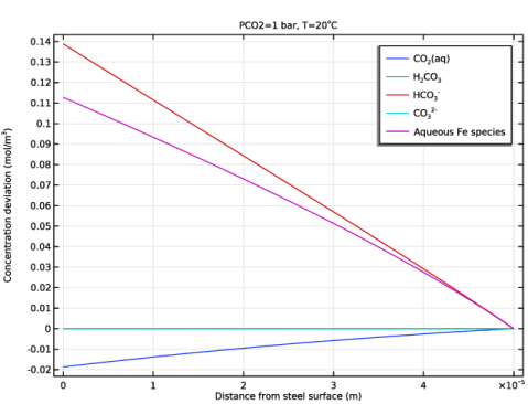
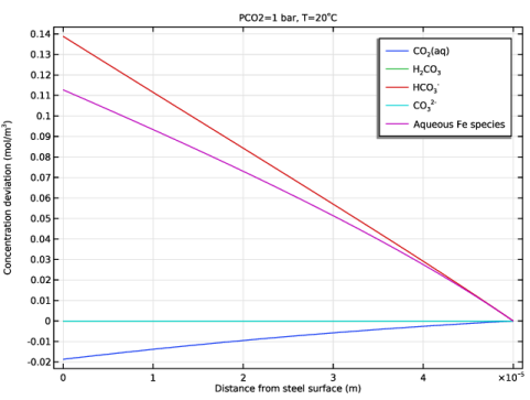
Select the x-axis label checkbox. In the associated text field, type Distance from steel surface (m).
10
Select the y-axis label checkbox. In the associated text field, type Concentration deviation (mol/m<sup>3</sup>).
Line Graph 1
1
Right-click Concentrations and choose Line Graph.
2
In the Settings window for Line Graph, locate the Selection section.
3
From the Selection list, choose All domains.
4
Locate the y-Axis Data section. In the Expression text field, type aqt.c4_H2CO3-intop_bulk(aqt.c4_H2CO3).
5
Click to expand the Title section. From the Title type list, choose None.
6
Locate the x-Axis Data section. From the Parameter list, choose Expression.
7
In the Expression text field, type x.
8
Click to expand the Legends section. Select the Show legends checkbox.
9
From the Legends list, choose Manual.
10
Line Graph 2
1
Right-click Line Graph 1 and choose Duplicate.
2
In the Settings window for Line Graph, locate the y-Axis Data section.
3
In the Expression text field, type aqt.c3_H2CO3-intop_bulk(aqt.c3_H2CO3).
4
Locate the Legends section. In the table, enter the following settings:
Line Graph 3
1
Right-click Line Graph 2 and choose Duplicate.
2
In the Settings window for Line Graph, locate the y-Axis Data section.
3
In the Expression text field, type aqt.c2_H2CO3-intop_bulk(aqt.c2_H2CO3).
4
Locate the Legends section. In the table, enter the following settings:
Line Graph 4
1
Right-click Line Graph 3 and choose Duplicate.
2
In the Settings window for Line Graph, locate the y-Axis Data section.
3
In the Expression text field, type aqt.c1_H2CO3-intop_bulk(aqt.c1_H2CO3).
4
Locate the Legends section. In the table, enter the following settings:
Line Graph 5
1
Right-click Line Graph 4 and choose Duplicate.
2
In the Settings window for Line Graph, locate the y-Axis Data section.
3
In the Expression text field, type aqt.c_Fe-intop_bulk(aqt.c_Fe).
4
Locate the Legends section. In the table, enter the following settings:
5
In the Concentrations toolbar, click  Plot.
Corrosion rate
1
In the Results toolbar, click  1D Plot Group.
2
In the Settings window for 1D Plot Group, type Corrosion rate in the Label text field.
3
Locate the Data section. From the Dataset list, choose Study 1/Solution 1 (sol1).
4
Locate the Title section. From the Title type list, choose None.
5
Locate the Plot Settings section.
6
Select the x-axis label checkbox. In the associated text field, type Partial pressure of CO2 (bar).
7
Select the y-axis label checkbox. In the associated text field, type Corrosion rate (mm/year).
8
Locate the Legend section. From the Position list, choose Upper left.
Point Graph 1
1
Right-click Corrosion rate and choose Point Graph.
2
3
In the Settings window for Point Graph, click Replace Expression in the upper-right corner of the y-Axis Data section. From the menu, choose Component 1 (comp1) > Aqueous Electrolyte Transport > Dissolving–depositing species > aqt.vtot - Total growth velocity - m/s.
4
Locate the y-Axis Data section. In the Expression text field, type -aqt.vtot.
5
From the Unit list, choose mm/yr.
6
Locate the x-Axis Data section. From the Axis source data list, choose PCO2.
7
From the Parameter list, choose Expression.
8
In the Expression text field, type PCO2.
9
Click to expand the Legends section. Select the Show legends checkbox.
10
From the Legends list, choose Evaluated.
11
In the Legend text field, type T=eval(T) K.
Corrosion rate
1
In the Model Builder window, click Corrosion rate.
2
In the Corrosion rate toolbar, click  Plot.
pH at surface
1
Right-click Corrosion rate and choose Duplicate.
2
In the Settings window for 1D Plot Group, type pH at surface in the Label text field.
3
Locate the Plot Settings section. In the y-axis label text field, type pH at surface.
4
Locate the Legend section. From the Position list, choose Upper right.
Point Graph 1
1
In the Model Builder window, expand the pH at surface node, then click Point Graph 1.
2
In the Settings window for Point Graph, locate the y-Axis Data section.
3
In the Expression text field, type aqt.pH.
pH at surface
1
In the Model Builder window, click pH at surface.
2
In the pH at surface toolbar, click  Plot.
pH at bulk
1
Right-click pH at surface and choose Duplicate.
2
In the Settings window for 1D Plot Group, type pH at bulk in the Label text field.
3
Locate the Plot Settings section. In the y-axis label text field, type pH at bulk.
Point Graph 1
1
In the Model Builder window, expand the pH at bulk node, then click Point Graph 1.
2
In the Settings window for Point Graph, locate the Selection section.
3
Click to select the  Activate Selection toggle button.
4
5
6
In the pH at bulk toolbar, click  Plot.