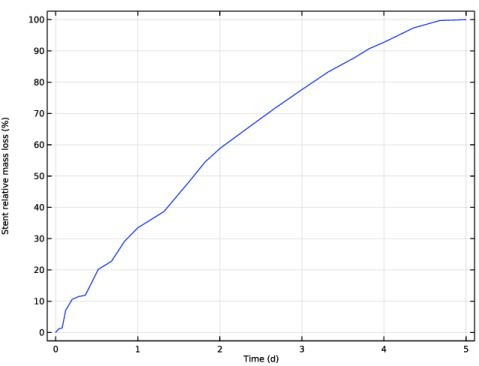
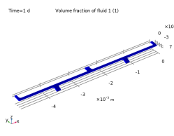
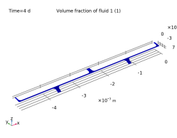
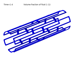
|
|
|



 |
|
 |
|
 |
 |
|
 |
 and
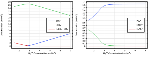
and  ions are set to 25 mol/m3 and 1 mol/m3, respectively.
|
1
|
|
2
|
|
3
|
Click Add.
|
|
4
|
Click
 Study. Study. |
|
5
|
In the Select Study tree, select Preset Studies for Selected Physics Interfaces > Time Dependent with Phase Initialization.
|
|
6
|
Click
 Done. Done. |
|
1
|
|
2
|
|
3
|
Click
 Load from File. Load from File. |
|
4
|
Browse to the model’s Application Libraries folder and double-click the file biodegradation_mg_stent_parameters.txt.
|
|
1
|
|
2
|
|
3
|
Click
 Browse. Browse. |
|
4
|
Browse to the model’s Application Libraries folder and double-click the file biodegradation_mg_stent.mphbin.
|
|
5
|
Click
 Import. Import. |
|
1
|
|
2
|
|
3
|
|
4
|
|
1
|
|
2
|
|
3
|
|
4
|
|
5
|
|
1
|
|
2
|
|
3
|
|
4
|
|
5
|
|
1
|
|
2
|
|
4
|
|
5
|
|
6
|
Click
 Build All Objects. Build All Objects. |
|
1
|
|
2
|
|
3
|
|
1
|
|
2
|
|
3
|
|
1
|
|
2
|
In the Settings window for Global Variable Probe, type stent_mass_loss in the Variable name text field.
|
|
3
|
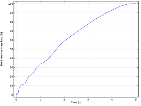
Locate the Expression section. In the Expression text field, type 1-intop1(phils>0.5)/at(0,intop1(phils>0.5)).
|
|
4
|
|
5
|
|
1
|
|
2
|
|
1
|
|
2
|
|
1
|
|
2
|
|
1
|
|
2
|
|
3
|
|
4
|
|
5
|
Click OK.
|
|
1
|
|
2
|
|
3
|
|
4
|
|
5
|
|
1
|
|
2
|
|
3
|
|
1
|
|
2
|
|
3
|
From the list, choose User-controlled mesh.
|
|
1
|
|
2
|
|
3
|
Clear the Minimum element size checkbox.
|
|
1
|
|
2
|
|
3
|
Click
 Paste Selection. Paste Selection. |
|
4
|
|
5
|
Click OK.
|
|
1
|
|
2
|
|
3
|
Click the Custom button.
|
|
4
|
Locate the Element Size Parameters section.
|
|
5
|
|
6
|
|
1
|
|
2
|
|
3
|
|
4
|
|
1
|
|
2
|
|
3
|
|
1
|
|
2
|
|
3
|
|
4
|
|
1
|
|
2
|
|
3
|
Click
 Paste Selection. Paste Selection. |
|
4
|
|
5
|
Click OK.
|
|
6
|
|
7
|
|
8
|
|
9
|
|
10
|
|
1
|
|
2
|
|
3
|
|
1
|
|
2
|
|
3
|
|
4
|
|
1
|
|
2
|
|
3
|
|
4
|
|
5
|
|
1
|
|
2
|
|
3
|
|
4
|
|
1
|
|
2
|
|
3
|
Clear the Plot dataset edges checkbox.
|
|
4
|
|
1
|
|
2
|
|
1
|
|
2
|
|
3
|
|
1
|
|
2
|
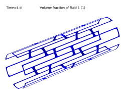
In the Settings window for 3D Plot Group, type Stent Shape in Model Geometry in the Label text field.
|
|
3
|
|
4
|
|
5
|
|
6
|
|
1
|
|
2
|
|
3
|
|
1
|
|
2
|
|
3
|
|
4
|
|
5
|
|
6
|
|
1
|
|
2
|
|
3
|
|
1
|
|
2
|
|
3
|
|
4
|
|
5
|
|
6
|
|
1
|
|
2
|
|
3
|
|
4
|
|
5
|
|
6
|
|
7
|
|
8
|
|
9
|
|
10
|
|
1
|
|
2
|
Go to the Add Physics window.
|
|
3
|
|
4
|
Find the Physics interfaces in study subsection. In the table, clear the Solve checkbox for Study 1.
|
|
5
|
Click the Add to Component 1 button in the window toolbar.
|
|
6
|
|
1
|
|
2
|
|
3
|
|
4
|
Browse to the model’s Application Libraries folder and double-click the file biodegradation_mg_stent_acid_equilibria_parameters.txt.
|
|
1
|
|
2
|
|
3
|
|
4
|
|
1
|
|
2
|
|
3
|
|
4
|
|
5
|
|
6
|
Browse to the model’s Application Libraries folder and double-click the file biodegradation_mg_stent_vessel_variables.txt.
|
|
1
|
|
2
|
|
3
|
|
4
|
|
5
|
|
6
|
Browse to the model’s Application Libraries folder and double-click the file biodegradation_mg_stent_tissue_stent_variables.txt.
|
|
1
|
|
2
|
|
3
|
Clear the Solve for electrolyte phase potential checkbox.
|
|
4
|
Select the Convection checkbox.
|
|
1
|
In the Model Builder window, under Component 1 (comp1) > Aqueous Electrolyte Transport (aqt) click Electrolyte 1.
|
|
2
|
|
3
|
Specify the u vector as
|
|
4
|
|
1
|
|
2
|
|
3
|
|
4
|
From the list, choose Polyprotic.
|
|
6
|
Select the Immobile species checkbox.
|
|
7
|
|
1
|
|
1
|
|
2
|
|
3
|
|
4
|
From the list, choose Polyprotic.
|
|
6
|
Select the Immobile species checkbox.
|
|
7
|
|
1
|
In the Settings window for Fully Dissociated Species, type Fully Dissociated Species: Mg in the Label text field.
|
|
2
|
|
3
|
|
4
|
|
1
|
In the Model Builder window, under Component 1 (comp1) > Aqueous Electrolyte Transport (aqt) click Initial Values 1.
|
|
2
|
|
3
|
|
1
|
|
2
|
|
3
|
|
4
|
|
5
|
|
1
|
|
3
|
|
4
|
|
5
|
|
1
|
|
1
|
|
1
|
|
2
|
In the Settings window for Fully Dissociated Species, type Fully Dissociated Species: Auxiliary Ions in the Label text field.
|
|
3
|
|
4
|
|
5
|
Select the Immobile species checkbox.
|
|
6
|
|
1
|
|
2
|
|
3
|
|
4
|
|
1
|
|
2
|
Go to the Add Study window.
|
|
3
|
Find the Studies subsection. In the Select Study tree, select Preset Studies for Some Physics Interfaces > Stationary.
|
|
4
|
Find the Physics interfaces in study subsection. In the table, clear the Solve checkbox for Level Set (ls).
|
|
5
|
Click the Add Study button in the window toolbar.
|
|
6
|
|
1
|
|
2
|
|
3
|
Click
 Add. Add. |
|
5
|
|
1
|
|
2
|
|
3
|
Find the Values of variables not solved for subsection. From the Settings list, choose User controlled.
|
|
4
|
|
5
|
|
6
|
|
7
|
|
8
|
|
9
|
|
10
|
Clear the Generate default plots checkbox.
|
|
11
|
|
1
|
|
2
|
|
3
|
|
4
|
|
5
|
|
1
|
|
2
|
|
3
|
|
4
|
|
5
|
|
6
|
|
7
|
|
8
|
|
9
|
|
1
|
|
2
|
|
3
|
|
4
|
|
5
|
|
1
|
|
2
|
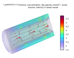
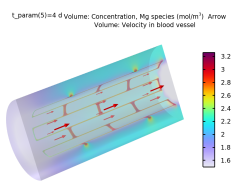
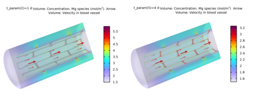
In the Settings window for Volume, click Replace Expression in the upper-right corner of the Expression section. From the menu, choose Component 1 (comp1) > Aqueous Electrolyte Transport > Fully Dissociated Species: Mg > aqt.c_Mg - Concentration, Mg species - mol/m³.
|
|
3
|
|
1
|
|
2
|
|
3
|
|
1
|
|
2
|
|
3
|
|
4
|
|
5
|
|
6
|
|
7
|
Locate the Arrow Positioning section. Find the x grid points subsection. In the Points text field, type 3.
|
|
1
|
|
2
|
|
3
|
|
4
|
|
5
|
|
6
|
|
7
|
|
8
|
|
1
|
|
2
|
|
1
|
|
2
|
|
3
|
|
1
|
|
2
|
|
3
|
|
4
|
|
5
|
|
6
|
|
7
|