|
|
|


|
1
|
|
2
|
|
3
|
Click Add.
|
|
4
|
Click
|
|
5
|
In the Select Study tree, select Preset Studies for Selected Physics Interfaces > Time Dependent with Initialization.
|
|
6
|
Click
|
|
1
|
|
2
|
|
3
|
Click
|
|
4
|
Browse to the model’s Application Libraries folder and double-click the file act_scratched_galvanized_steel_parameters.txt.
|
|
1
|
|
2
|
|
3
|
|
4
|
|
1
|
|
2
|
|
3
|
|
4
|
|
5
|
|
6
|
|
7
|
|
8
|
|
1
|
|
2
|
|
3
|
|
4
|
Click
|
|
1
|
|
2
|
|
3
|
|
4
|
|
1
|
|
2
|
|
3
|
|
4
|
|
5
|
|
1
|
|
2
|
|
3
|
|
4
|
|
5
|
|
6
|
Click
|
|
7
|
|
1
|
|
2
|
|
1
|
|
2
|
|
1
|
|
2
|
|
3
|
|
1
|
|
2
|
|
3
|
|
4
|
|
1
|
|
2
|
|
3
|
|
4
|
|
1
|
|
2
|
|
3
|
|
4
|
|
1
|
|
2
|
In the Settings window for Interpolation, type Interpolation - Relative Humidity in the Label text field.
|
|
3
|
|
4
|
Click
|
|
5
|
Browse to the model’s Application Libraries folder and double-click the file act_scratched_galvanized_steel_rh.txt.
|
|
6
|
Locate the Interpolation and Extrapolation section. From the Interpolation list, choose Piecewise cubic.
|
|
7
|
|
8
|
In the Argument table, enter the following settings:
|
|
1
|
|
2
|
|
3
|
|
4
|
Click
|
|
5
|
Browse to the model’s Application Libraries folder and double-click the file act_scratched_galvanized_steel_temperature.txt.
|
|
6
|
Locate the Interpolation and Extrapolation section. From the Interpolation list, choose Piecewise cubic.
|
|
7
|
|
8
|
In the Argument table, enter the following settings:
|
|
1
|
|
2
|
|
3
|
|
4
|
Click
|
|
5
|
Browse to the model’s Application Libraries folder and double-click the file act_scratched_galvanized_steel_spray.txt.
|
|
6
|
Locate the Interpolation and Extrapolation section. From the Interpolation list, choose Piecewise cubic.
|
|
7
|
|
8
|
In the Argument table, enter the following settings:
|
|
1
|
|
2
|
Go to the Add Material window.
|
|
3
|
|
4
|
Click the Add to Component button in the window toolbar.
|
|
5
|
|
6
|
Click the Add to Component button in the window toolbar.
|
|
7
|
|
1
|
|
2
|
|
1
|
|
2
|
|
3
|
|
1
|
|
2
|
|
3
|
|
4
|
Browse to the model’s Application Libraries folder and double-click the file act_scratched_galvanized_steel_global_variables.txt.
|
|
1
|
|
2
|
|
3
|
|
4
|
|
5
|
|
6
|
Browse to the model’s Application Libraries folder and double-click the file act_scratched_galvanized_steel_rate_variables.txt.
|
|
1
|
|
2
|
|
3
|
|
4
|
|
5
|
|
6
|
Browse to the model’s Application Libraries folder and double-click the file act_scratched_galvanized_steel_film_variables.txt.
|
|
1
|
|
2
|
|
3
|
|
4
|
|
5
|
|
6
|
Browse to the model’s Application Libraries folder and double-click the file act_scratched_galvanized_steel_zn_variables.txt.
|
|
1
|
|
2
|
|
3
|
|
4
|
|
5
|
|
6
|
Browse to the model’s Application Libraries folder and double-click the file act_scratched_galvanized_steel_fe_variables.txt.
|
|
1
|
|
2
|
In the Settings window for Aqueous Electrolyte Transport, locate the Out-of-Plane Thickness section.
|
|
3
|
|
1
|
In the Model Builder window, under Component 1 (comp1) > Aqueous Electrolyte Transport (aqt) click Electrolyte 1.
|
|
2
|
|
3
|
|
4
|
|
5
|
|
1
|
|
2
|
|
3
|
|
4
|
|
6
|
|
7
|
|
1
|
|
2
|
|
3
|
|
4
|
|
5
|
|
1
|
In the Settings window for Fully Dissociated Species, type Fully Dissociated Species - Na in the Label text field.
|
|
2
|
|
3
|
|
4
|
|
1
|
In the Settings window for Fully Dissociated Species, type Fully Dissociated Species - Cl in the Label text field.
|
|
2
|
|
3
|
|
4
|
|
1
|
In the Model Builder window, under Component 1 (comp1) > Aqueous Electrolyte Transport (aqt) click Initial Values 1.
|
|
2
|
|
3
|
|
4
|
|
5
|
|
6
|
|
1
|
|
2
|
In the Settings window for Highly Conductive Porous Electrode, type Highly Conductive Porous Electrode - Steel in the Label text field.
|
|
3
|
|
4
|
|
6
|
Clear the Subtract volume change from electrolyte volume fraction checkbox.
|
|
1
|
In the Model Builder window, expand the Highly Conductive Porous Electrode - Steel node, then click Porous Electrode Reaction 1.
|
|
2
|
|
3
|
|
4
|
|
5
|
Locate the Electrode Kinetics section. From the iloc,expr list, choose User defined. In the associated text field, type i_red.
|
|
6
|
|
1
|
|
2
|
|
3
|
|
4
|
|
5
|
Find the Stoichiometric coefficients for dissolving–depositing species subsection. In the table, enter the following settings:
|
|
1
|
|
2
|
In the Settings window for Highly Conductive Porous Electrode, type Highly Conductive Porous Electrode - Zinc in the Label text field.
|
|
3
|
|
4
|
|
6
|
Click
|
|
8
|
Clear the Subtract volume change from electrolyte volume fraction checkbox.
|
|
1
|
In the Model Builder window, expand the Highly Conductive Porous Electrode - Zinc node, then click Porous Electrode Reaction 1.
|
|
2
|
|
3
|
|
4
|
|
5
|
Find the Stoichiometric coefficients for dissolving–depositing species subsection. In the table, enter the following settings:
|
|
6
|
Locate the Electrode Kinetics section. From the iloc,expr list, choose User defined. In the associated text field, type i_ox.
|
|
7
|
|
1
|
|
2
|
|
3
|
|
4
|
|
5
|
Find the Stoichiometric coefficients for dissolving–depositing species subsection. In the table, enter the following settings:
|
|
1
|
|
2
|
In the Settings window for Species Source, type Species Source - Atmospheric Carbon Dioxide Dissolution in the Label text field.
|
|
3
|
|
4
|
|
1
|
|
2
|
|
3
|
|
4
|
|
5
|
|
6
|
|
7
|
|
8
|
|
9
|
|
10
|
|
11
|
|
12
|
|
13
|
|
14
|
|
15
|
|
16
|
|
1
|
|
2
|
|
3
|
|
4
|
|
5
|
|
6
|
|
7
|
Click to expand the Smoothing section.
|
|
8
|
|
9
|
|
1
|
|
2
|
In the Settings window for Global Variable Probe, type Global Variable Probe - ZnO in the Label text field.
|
|
3
|
|
4
|
|
5
|
|
6
|
Select the Description checkbox.
|
|
7
|
|
8
|
Click
|
|
1
|
|
2
|
In the Settings window for Global Variable Probe, type Global Variable Probe - Zinc Metal in the Label text field.
|
|
3
|
|
4
|
|
5
|
|
6
|
Select the Description checkbox.
|
|
7
|
|
8
|
|
1
|
|
2
|
In the Settings window for Global Variable Probe, type Global Variable Probe - Total Zinc Metal Dissolution Current in the Label text field.
|
|
3
|
|
4
|
|
5
|
|
6
|
Select the Description checkbox.
|
|
7
|
|
8
|
Click
|
|
1
|
|
2
|
In the Settings window for Global Variable Probe, type Global Variable Probe - Total Oxygen Reduction Current in the Label text field.
|
|
3
|
|
4
|
|
5
|
|
6
|
Select the Description checkbox.
|
|
7
|
|
8
|
|
1
|
|
2
|
In the Settings window for Domain Probe, type Domain Probe - Maximum Zinc Coating Thickness Loss in the Label text field.
|
|
3
|
|
4
|
|
5
|
|
6
|
|
7
|
|
8
|
Select the Description checkbox.
|
|
9
|
|
10
|
Click
|
|
1
|
|
2
|
|
3
|
|
4
|
|
5
|
|
6
|
Click
|
|
1
|
|
2
|
|
3
|
|
4
|
|
1
|
|
2
|
In the Settings window for Domain Probe, type Domain Probe - Average NaCl Concentration in Liquid Film in the Label text field.
|
|
3
|
|
4
|
|
5
|
|
6
|
Click
|
|
1
|
|
2
|
|
3
|
|
1
|
|
2
|
|
3
|
|
4
|
|
1
|
|
2
|
|
3
|
|
4
|
|
5
|
|
6
|
|
1
|
|
2
|
|
3
|
|
4
|
Locate the Plot Settings section.
|
|
5
|
|
6
|
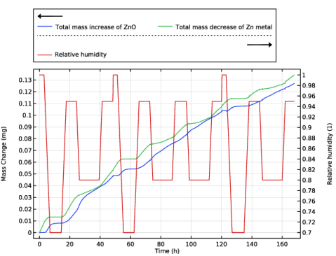
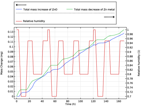
Select the Two y-axes checkbox.
|
|
7
|
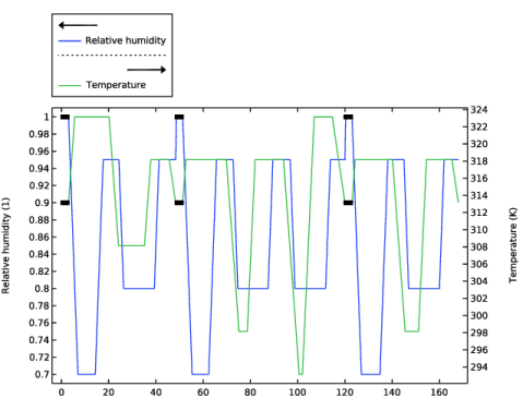
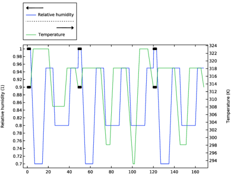
Select the Secondary y-axis label checkbox. In the associated text field, type Relative humidity (1).
|
|
8
|
|
9
|
|
1
|
In the Model Builder window, expand the Mass Change on Full Sample node, then click Probe Table Graph 1.
|
|
2
|
|
3
|
|
1
|
|
2
|
|
3
|
|
4
|
|
5
|
|
6
|
Locate the y-Axis Data section. In the table, enter the following settings:
|
|
7
|
|
9
|
|
1
|
|
2
|
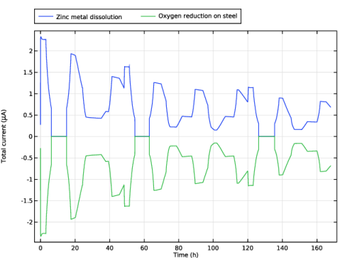
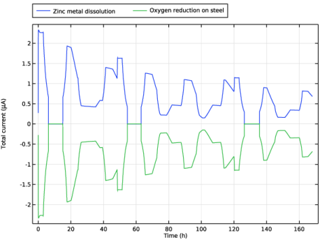
In the Settings window for 1D Plot Group, type Total Current on Full Sample in the Label text field.
|
|
3
|
Locate the Plot Settings section.
|
|
4
|
|
5
|
|
6
|
|
1
|
In the Model Builder window, expand the Total Current on Full Sample node, then click Probe Table Graph 1.
|
|
2
|
|
3
|
|
5
|
|
1
|
|
2
|
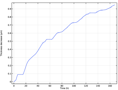
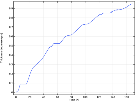
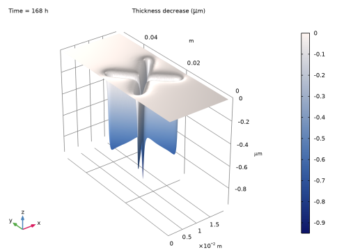
In the Settings window for 1D Plot Group, type Maximum Decrease Coating Thickness in the Label text field.
|
|
3
|
Locate the Plot Settings section.
|
|
4
|
|
5
|
|
6
|
|
1
|
|
2
|
|
3
|
Locate the Plot Settings section.
|
|
4
|
|
5
|
|
6
|
|
1
|
|
2
|
|
3
|
|
5
|
|
1
|
|
2
|
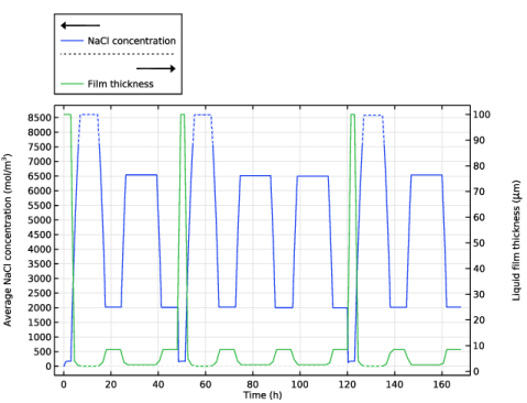
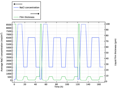
In the Settings window for 1D Plot Group, type Average NaCl Concentration and Liquid Film Thickness in the Label text field.
|
|
3
|
|
4
|
Locate the Plot Settings section.
|
|
5
|
Select the y-axis label checkbox. In the associated text field, type Average NaCl concentration (mol/m<sup>3</sup>).
|
|
6
|
Select the Two y-axes checkbox.
|
|
7
|
Select the Secondary y-axis label checkbox. In the associated text field, type Liquid film thickness (\mu m).
|
|
8
|
|
9
|
|
10
|
|
1
|
In the Model Builder window, expand the Average NaCl Concentration and Liquid Film Thickness node, then click Probe Table Graph 1.
|
|
2
|
|
3
|
|
1
|
|
2
|
|
3
|
|
4
|
|
5
|
Locate the Coloring and Style section. Find the Line style subsection. From the Line list, choose Dotted.
|
|
6
|
|
7
|
|
1
|
|
2
|
|
3
|
|
4
|
Locate the y-Axis Data section. In the table, enter the following settings:
|
|
5
|
|
1
|
Right-click Results > Average NaCl Concentration and Liquid Film Thickness > Global 1 and choose Duplicate.
|
|
2
|
|
3
|
|
4
|
|
5
|
|
1
|
|
2
|
|
3
|
|
4
|
|
1
|
|
2
|
|
3
|
|
4
|
|
5
|
|
6
|
|
7
|
|
8
|
Select the Two y-axes checkbox.
|
|
9
|
|
10
|
|
11
|
|
12
|
|
1
|
|
2
|
|
4
|
|
1
|
|
2
|
|
3
|
|
4
|
|
5
|
|
6
|
|
1
|
|
2
|
|
3
|
|
1
|
|
2
|
Right-click and choose Duplicate.
|
|
1
|
|
2
|
Select the Plot on secondary y-axis checkbox.
|
|
3
|
Locate the y-Axis Data section. In the table, enter the following settings:
|
|
4
|
Locate the Legends section. In the table, enter the following settings:
|
|
1
|
|
2
|
|
3
|
Select the Plot on secondary y-axis checkbox.
|
|
4
|
Locate the y-Axis Data section. In the table, enter the following settings:
|
|
5
|
|
1
|
|
2
|
|
3
|
|
4
|
|
5
|
|
6
|
|
1
|
|
2
|
|
3
|
|
4
|
|
5
|
|
6
|
Clear the Parameter indicator text field.
|
|
7
|
|
8
|
|
1
|
|
2
|
|
3
|
|
4
|
|
5
|
|
6
|
|
7
|
|
8
|
|
9
|
|
1
|
|
2
|
|
3
|
Clear the Show height axis checkbox.
|
|
1
|
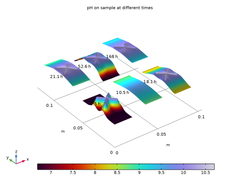
In the Model Builder window, under Results > pH Full Sample right-click Surface 1 and choose Duplicate.
|
|
2
|
|
3
|
|
4
|
|
1
|
|
2
|
|
3
|
|
1
|
|
2
|
|
3
|
|
1
|
|
2
|
|
3
|
|
1
|
|
2
|
|
3
|
|
4
|
|
1
|
|
2
|
|
3
|
|
4
|
|
5
|
|
6
|
|
7
|
|
8
|
|
9
|
|
10
|
|
11
|
|
12
|
|
1
|
|
2
|
|
3
|
|
4
|
|
5
|
|
1
|
|
2
|
|
3
|
|
4
|
|
1
|
|
2
|
|
3
|
|
4
|
|
5
|
|
1
|
|
2
|
|
3
|
|
4
|
|
1
|
|
2
|
|
3
|
|
4
|
|
5
|
|
6
|
|
1
|
|
2
|
|
3
|
|
4
|
|
5
|
|
6
|
|
7
|
|
1
|
|
2
|
|
3
|
|
4
|
|
5
|
|
6
|
|
7
|
|
8
|
|
1
|
|
2
|
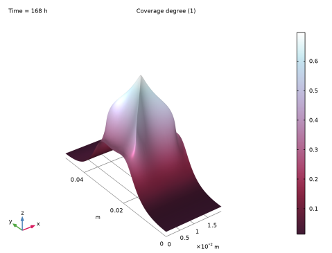
In the Settings window for 2D Plot Group, type Corrosion Product Coverage Degree in the Label text field.
|
|
3
|
|
4
|
|
5
|
|
6
|
|
7
|
|
1
|
|
2
|
|
3
|
|
4
|
|
5
|
|
1
|
|
2
|
|
3
|
Clear the Show height axis checkbox.
|
|
4
|
|
5
|