PDF

Stress and Modal Analysis of a Wind Turbine Composite Blade
Introduction
Wind turbines are an increasingly popular source of renewable energy. As such, the design, analysis and manufacture of wind turbines are important to the energy industry.
The turbine blades are critical components of a wind turbine. When generating electric power through rotation, they have to withstand different types of loads, such as wind, gravitational, and centrifugal loads. The sheer size of a blade necessitates light and strong materials, and composites are well suited for this.
This example shows how to analyze a composite wind turbine blade using a mixture of carbon–epoxy, glass–vinylester and PVC foam. The blade is constructed as a sandwich structure where the PVC foam core is sandwiched between carbon–epoxy and glass–vinylester.
First, a stress analysis of the blade is performed in which it is subjected to a combination of gravitational and centrifugal loads. The tip displacement, maximum stress values, and through-thickness stress distribution at a particular point on the blade are computed for different load cases. Second, a prestressed eigenfrequency analysis is performed for a range of operating speeds. A Campbell diagram depicting the variation of eigenfrequencies with rotation speed is generated.
Model Definition
The geometry consists of a wind turbine blade of 61.5 m length as shown in Figure 1. This is a blade geometry used in the NREL 5MW wind turbine (Ref. 1 and Ref. 2). The front and top views of the geometry are shown in Figure 2.
The blade geometry has 19 different sections, where each section is defined by an airfoil shape. The details of the type of airfoil together with the maximum chord and the twist in each section is given in Table 1.
Essentially there are six different types of airfoils which are used to build the full wind turbine blade as shown in Figure 3. Note that the NACA 64-618 is the best airfoil from aerodynamic point of view and hence used near the tip region whereas the DU 99-W-405 is good from a structural point of view and hence used near the root of the blade. In between there are other airfoils of DU family which are used for smooth transition between the two extreme airfoil shapes. More details about the DU family airfoils can be found in Ref. 3.
Figure 1: Geometry of a wind turbine blade for the NREL 5MW wind turbine. The different airfoils used at various sections are also shown.
Figure 2: Front view (zx-plane) and top view (xy-plane) of the wind turbine blade.
There are two important parts of a wind turbine blade:
The skin consists of the outer curved boundaries. It carries essentially the entire loading. In order to increase bending and torsional stiffness, the blade is reinforced using spars, which are internal vertical members.
Figure 3: Different types of airfoils used at various sections of the wind turbine blade.
Loads and Boundary Conditions
The left end of the blade is connected to the rotor hub, and it is fixed, as shown in Figure 4. The loads acting on the structure are the self-weight of the blade and the centrifugal force. The aerodynamic or wind loads are not considered.
Two types of analyses are performed:
Figure 4: The geometry showing boundary conditions and loads acting on the structure.
lamina Material Properties
The analyzed wind turbine blade is a sandwich structure consisting of three different layered material types as shown in Figure 5.
The material properties of different laminae is taken from Ref. 4.
Figure 5: Sandwich arrangement of different layered materials used in the skin as well as in the spar of the blade.
Carbon–Epoxy Laminate
The outer part of the sandwich structure is a carbon–epoxy laminate having 10 layers, each of thickness 0.28 mm and oriented at 0 degrees to the first axis of the laminate coordinate system. The density of the lamina is taken as 1560 kg/m3. The transversely isotropic material properties of the lamina are given in Table 2.
{E11,E22}
G12
{υ12,υ23}
Glass–Vinylester Laminate
The next part of the sandwich structure is a glass–vinylester laminate. The density of this lamina is taken as 1890 kg/m3. The transversely isotropic material properties are given in Table 3.
{E11,E22}
G12
{υ12,υ23}
This laminate is made of 40 layers, each of 0.28 mm thickness with the stacking sequence shown in Table 4 and Figure 6.
Figure 6: Stacking sequence of the glass–vinylester laminate, showing the fiber orientation in each layer, from bottom to top.
PVC Foam
The core material of the sandwich structure is made of PVC Foam of thickness 15 cm. The density of the material is taken as 200 kg/m3. The values of Young’s modulus, shear modulus and Poisson’s ratio for the material are taken as 250 MPa, 92.6 MPa, and 0.35, respectively.
Laminate Coordinate System
The orientation of the laminate coordinate system in which the laminate material properties are specified is shown in Figure 7.
Figure 7: The laminate coordinate system used to define material properties in the wind turbine blade.
Finite Element Mesh
The structure is discretized using a mapped mesh, as shown in Figure 8.
Figure 8: The mapped mesh for the wind turbine blade.
Results and Discussion
Figure 9: The stress distribution in the skin and spar for combined gravitational and centrifugal loads.
Figure 10: The stress distribution in the spars for combined gravitational and centrifugal loads.
Figure 9 shows the distribution of stress in the fiber direction in each layer of the skin and spars for a combined load case of gravitational and centrifugal forces. High stresses are present near the root of the blade and in the junction between the circular and airfoil cross sections. The stress distribution for the spars is shown separately in Figure 10. The stress distribution in the outermost carbon–epoxy laminate is shown in Figure 11 for the three load cases.
Figure 11: The stress distribution in the outermost carbon–epoxy layer for the three different load cases.
Figure 12: The fourth mode shape of the blade for different blade speeds.
Figure 13: First six mode shapes of the blade when it is not rotating.
In the second part of the example, a prestressed eigenfrequency analysis is carried out to compute eigenfrequencies and corresponding mode shapes of the blade under centrifugal forces. Different mode shapes of the blade as well as the effect of centrifugal force on the mode shape are shown in Figure 12 and Figure 13.
A Campbell plot is created in order to understand the variation of eigenfrequencies with respect to the blade rotation speed as shown in Figure 14. The eigenfrequencies increase with an increase in the blade RPM. This is due to the centrifugal stiffening effect.
Figure 14: Campbell plot showing the variation of eigenfrequencies with an increase in the blade RPM.
Notes About the COMSOL Implementation
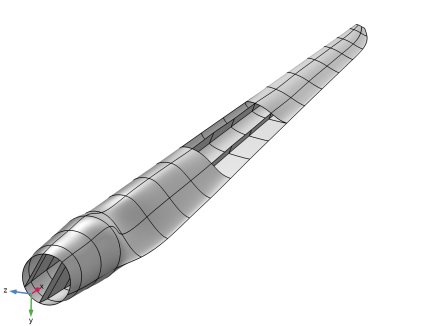
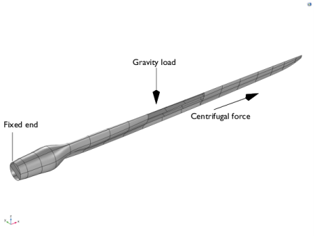
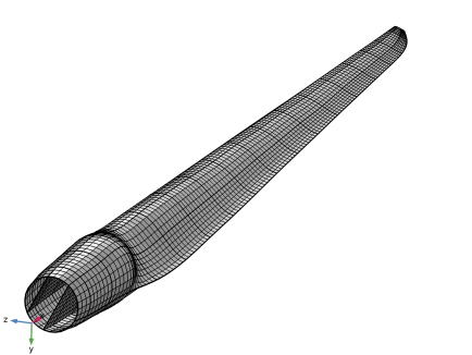
Modeling a composite laminate as a layered shell requires a surface geometry, in general referred to as a base surface, and a Layered Material node which adds an extra dimension (1D) to the base surface geometry in the surface normal direction. You can use the Layered Material functionality to model several layers stacked on top of each other having different thicknesses, material properties, and fiber orientations. You can optionally specify the interface materials between the layers, and control the number of through-thickness mesh elements for each layer.
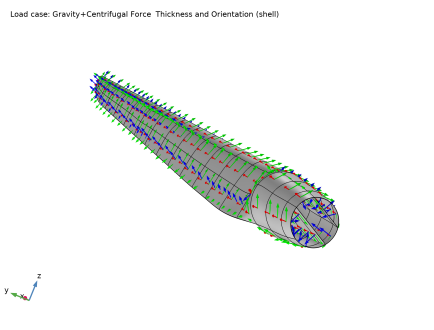
The third direction for the selected coordinate system in the Single Layer Material, Layered Material Link, or Layered Material Stack represents the normal direction of the Layered Shell or Shell physics. This is also the direction in which the layer stacking is interpreted from bottom to top, and therefore, it is crucial to know it during modeling. There are two ways to achieve this:
-
Using physics symbols: Go to the physics settings, find the Physics Symbols section, and select the Enable physics symbols checkbox. Then go to the material feature, for instance, Linear Elastic Material, to see the normal direction represented by green arrows in the geometry.
-
From a constitutive model point of view, you can either use the Layerwise (LW) theory based Layered Shell interface, or the Equivalent Single Layer (ESL) theory based Linear Elastic Material, Layered node in the Shell interface. The laminated composite presented in the current model is modeled using a Linear Elastic Material, Layered node in the Shell interface.
The built-in Composites material library contains data for fiber and matrix constituents as well as for unidirectional and bidirectional laminae.
References
1. J. Jonkman and others, Definition of a 5-MW Reference Wind Turbine for Offshore System Development, Technical Report, NREL/TP-500-38060, 2009.
2. M.K. Yeh, and C.H. Wang, Stress Analysis of Composite Wind Turbine Blade with Different Stacking Angle and Different Skin Thickness, ICMSEA and MCEBM, 2017.
3. W.A. Timmer and R.P.J.O.M. van Rooij, “Summary of the Delft University Wind Turbine Dedicated Airfoils,” J. Sol. Energy Eng., vol. 125, no. 4, pp. 488-496, 2003.
4. K. Kox and A. Echtermeyer, “Structural Design and Analysis of a 10MW Wind Turbine Blade,” Energy Procedia, vol. 24, pp. 194–201, 2012.
Application Library path: Composite_Materials_Module/Dynamics_and_Vibration/wind_turbine_composite_blade
Modeling Instructions
From the File menu, choose New.
New
In the New window, click  Model Wizard.
Model Wizard
1
In the Model Wizard window, click  3D.
2
In the Select Physics tree, select Structural Mechanics > Shell (shell).
3
Click Add.
4
Click  Study.
5
In the Select Study tree, select General Studies > Stationary.
6
Global Definitions
Parameters 1
1
In the Model Builder window, under Global Definitions click Parameters 1.
2
In the Settings window for Parameters, locate the Parameters section.
3
Geometry 1
Import 1 (imp1)
1
In the Model Builder window, expand the Component 1 (comp1) > Geometry 1 node.
2
Right-click Geometry 1 and choose Import.
3
In the Settings window for Import, locate the Source section.
4
From the Source list, choose COMSOL Multiphysics file.
5
Click  Browse.
6
7
Click  Import.
You can adjust the view of the geometry for better visualization.
Definitions
Skin Boundaries
1
In the Definitions toolbar, click  Explicit.
2
In the Settings window for Explicit, type Skin Boundaries in the Label text field.
3
Locate the Input Entities section. From the Geometric entity level list, choose Boundary.
4
5
Select the Group by continuous tangent checkbox.
Spar Boundaries
1
In the Definitions toolbar, click  Explicit.
2
In the Settings window for Explicit, type Spar Boundaries in the Label text field.
3
Locate the Input Entities section. From the Geometric entity level list, choose Boundary.
4
5
Select the Group by continuous tangent checkbox.
Fixed Edges
1
In the Definitions toolbar, click  Explicit.
2
In the Settings window for Explicit, type Fixed Edges in the Label text field.
3
Locate the Input Entities section. From the Geometric entity level list, choose Edge.
4
5
Select the Group by continuous tangent checkbox.
Average 1 (aveop1)
1
In the Definitions toolbar, click  Nonlocal Couplings and choose Average.
2
In the Settings window for Average, locate the Source Selection section.
3
From the Geometric entity level list, choose Edge.
4
From the Selection list, choose Fixed Edges.
5
Locate the Advanced section. From the Frame list, choose Material  (X, Y, Z).
Boundary System 1 (sys1)
1
In the Model Builder window, click Boundary System 1 (sys1).
2
In the Settings window for Boundary System, locate the Settings section.
3
Find the Coordinate names subsection. From the Axis list, choose x.
Reverse Normal 1
1
Right-click Boundary System 1 (sys1) and choose Reverse Normal.
2
In the Settings window for Reverse Normal, locate the Boundary Selection section.
3
From the Selection list, choose Skin Boundaries.
Geometry 1
1
In the Model Builder window, under Component 1 (comp1) click Geometry 1.
2
In the Graphics window toolbar, clicknext to  Select Objects, then choose Select Boundaries.
3
Click the  Click and Hide button in the Graphics toolbar.
You can hide parts of the skin to visualize the spars inside the blade.
Global Definitions
Material: Carbon–Epoxy
1
In the Model Builder window, under Global Definitions right-click Materials and choose Blank Material.
2
In the Settings window for Material, type Material: Carbon-Epoxy in the Label text field.
Layered Material: CE-[0]_10
1
Right-click Materials and choose Layered Material.
2
In the Settings window for Layered Material, type Layered Material: CE-[0]_10 in the Label text field.
3
Locate the Layer Definition section. In the table, enter the following settings:
Material: Glass–Vinylester
1
Right-click Materials and choose Blank Material.
2
In the Settings window for Material, type Material: Glass-Vinylester in the Label text field.
Layered Material: GV-[0/45/-45/90]_s_5
1
Right-click Materials and choose Layered Material.
2
In the Settings window for Layered Material, type Layered Material: GV-[0/45/-45/90]_s_5 in the Label text field.
3
Locate the Layer Definition section. In the table, enter the following settings:
4
Click Add seven times.
5
6
Click to expand the Preview Plot Settings section. In the Thickness-to-width ratio text field, type 0.6.
7
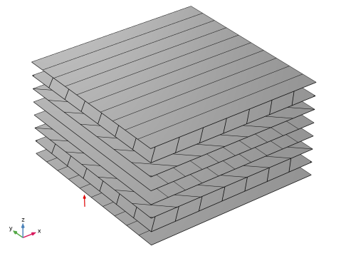
Locate the Layer Definition section. Click Layer Stack Preview in the upper-right corner of the section.
Material: PVC Foam
1
Right-click Materials and choose Blank Material.
2
In the Settings window for Material, type Material: PVC Foam in the Label text field.
Layered Material: PF-[0]
1
Right-click Materials and choose Layered Material.
2
In the Settings window for Layered Material, type Layered Material: PF-[0] in the Label text field.
3
Locate the Layer Definition section. In the table, enter the following settings:
Materials
Create a Layered Material Stack in which the previously created layered materials can be arranged to finalize the sandwich structure of the composite.
Layered Material Stack 1 (stlmat1)
In the Model Builder window, under Component 1 (comp1) right-click Materials and choose Layers > Layered Material Stack.
Layered Material Link: Carbon–Epoxy
In the Settings window for Layered Material Link, type Layered Material Link: Carbon-Epoxy in the Label text field.
Layered Material Link: Glass–Vinylester
1
Right-click Layered Material Link: Carbon–Epoxy and choose Duplicate.
2
In the Settings window for Layered Material Link, type Layered Material Link: Glass-Vinylester in the Label text field.
3
Locate the Link Settings section. From the Material list, choose Layered Material: GV-[0/45/-45/90]_s_5 (lmat2).
Layered Material Link: PVC Foam
1
Right-click Layered Material Link: Glass–Vinylester and choose Duplicate.
2
In the Settings window for Layered Material Link, type Layered Material Link: PVC Foam in the Label text field.
3
Locate the Link Settings section. From the Material list, choose Layered Material: PF-[0] (lmat3).
Layered Material Link: Glass–Vinylester 1 (stlmat1.stllmat4)
In the Model Builder window, under Component 1 (comp1) > Materials > Layered Material Stack 1 (stlmat1) right-click Layered Material Link: Glass–Vinylester (stlmat1.stllmat2) and choose Duplicate.
Layered Material Link: Carbon–Epoxy 1 (stlmat1.stllmat5)
In the Model Builder window, under Component 1 (comp1) > Materials > Layered Material Stack 1 (stlmat1) right-click Layered Material Link: Carbon–Epoxy (stlmat1.stllmat1) and choose Duplicate.
Layered Material Stack 1 (stlmat1)
1
In the Settings window for Layered Material Stack, click Section_bar in the upper-right corner of the Layered Material Settings section. From the menu, choose Layer Stack Preview.
2
Click to expand the Preview Plot Settings section. In the Thickness-to-width ratio text field, type 0.4.
3
Clear the Shows labels in cross-section plot checkbox.
4
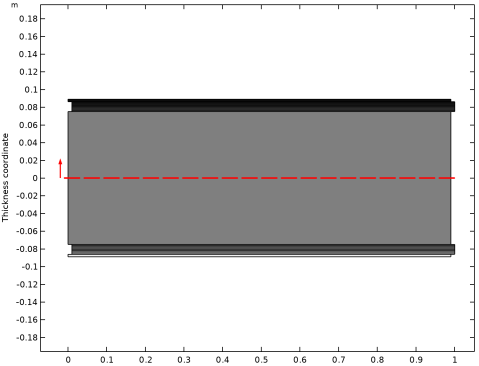
Locate the Layered Material Settings section. Click Layer Cross-Section Preview in the upper-right corner of the section.
Shell (shell)
Linear Elastic Material, Layered 1
1
In the Physics toolbar, click  Boundaries and choose Linear Elastic Material, Layered.
2
In the Settings window for Linear Elastic Material, Layered, locate the Boundary Selection section.
3
From the Selection list, choose All boundaries.
4
Locate the Linear Elastic Material section. From the Material symmetry list, choose Orthotropic.
5
Select the Transversely isotropic checkbox.
Add the material properties of carbon–epoxy, glass–vinylester and PVC foam.
Global Definitions
Material: Carbon–Epoxy (mat1)
1
In the Model Builder window, under Global Definitions > Materials click Material: Carbon–Epoxy (mat1).
2
In the Settings window for Material, locate the Material Contents section.
3
Material: Glass–Vinylester (mat2)
1
In the Model Builder window, click Material: Glass–Vinylester (mat2).
2
In the Settings window for Material, locate the Material Contents section.
3
Material: PVC Foam (mat3)
The PVC foam is isotropic. You just need to set the Young’s modulus and Poisson’s ratio. Orthotropic material properties will be synchronized from them.
1
In the Model Builder window, click Material: PVC Foam (mat3).
2
In the Settings window for Material, click to expand the Material Properties section.
3
In the Material properties tree, select Solid Mechanics > Linear Elastic Material > Young’s Modulus and Poisson’s Ratio.
4
Click  Add to Material.
5
Locate the Material Contents section. In the table, enter the following settings:
6
Click the  Show More Options button in the Model Builder toolbar.
7
In the Show More Options dialog, in the tree, select the checkbox for the node Physics > Advanced Physics Options.
8
Shell (shell)
Linear Elastic Material, Layered 1
1
In the Model Builder window, under Component 1 (comp1) > Shell (shell) click Linear Elastic Material, Layered 1.
2
In the Settings window for Linear Elastic Material, Layered, click to expand the Shear Correction Factor section.
3
Fixed Constraint 1
1
In the Physics toolbar, click  Edges and choose Fixed Constraint.
2
In the Settings window for Fixed Constraint, locate the Edge Selection section.
3
From the Selection list, choose Fixed Edges.
Gravity 1
1
In the Physics toolbar, click  Global and choose Gravity.
2
Click  Load Group and choose New Load Group.
Global Definitions
Load Group: Gravity
1
In the Model Builder window, under Global Definitions > Load and Constraint Groups click Load Group 1.
2
In the Settings window for Load Group, type Load Group: Gravity in the Label text field.
3
In the Parameter name text field, type lgG.
Shell (shell)
Rotating Frame 1
1
In the Physics toolbar, click  Boundaries and choose Rotating Frame.
2
In the Settings window for Rotating Frame, locate the Rotating Frame section.
3
From the Axis of rotation list, choose User defined. Specify the rbp vector as
4
Specify the eax vector as
5
In the ωr text field, type omega.
6
Locate the Frame Acceleration Effect section. Clear the Spin softening checkbox.
7
In the Physics toolbar, click  Load Group and choose New Load Group.
Global Definitions
Load Group: Centrifugal Force
1
In the Model Builder window, under Global Definitions > Load and Constraint Groups click Load Group 2.
2
In the Settings window for Load Group, type Load Group: Centrifugal Force in the Label text field.
3
In the Parameter name text field, type lgCF.
Mesh 1
Mapped 1
1
In the Mesh toolbar, click  More Generators and choose Mapped.
2
In the Settings window for Mapped, locate the Boundary Selection section.
3
From the Selection list, choose All boundaries.
Size 1
1
Right-click Mapped 1 and choose Size.
2
In the Settings window for Size, click to expand the Element Size Parameters section.
3
Locate the Element Size section. Click the Custom button.
4
Locate the Element Size Parameters section.
5
Select the Maximum element size checkbox. In the associated text field, type 0.5.
6
In the Model Builder window, right-click Mesh 1 and choose Build All.
Study: Static
1
In the Model Builder window, click Study 1.
2
In the Settings window for Study, type Study: Static in the Label text field.
Step 1: Stationary
1
In the Model Builder window, under Study: Static click Step 1: Stationary.
2
In the Settings window for Stationary, click to expand the Study Extensions section.
3
Select the Define load cases checkbox.
4
Add two additional load cases.
5
6
In the Study toolbar, click  Compute.
Set default units for result presentation.
Results
Preferred Units 1
1
In the Results toolbar, click  Configurations and choose Preferred Units.
2
In the Settings window for Preferred Units, locate the Units section.
3
Click  Add Physical Quantity.
4
In the Physical Quantity dialog, select Solid Mechanics > Stress tensor (N/m^2) in the tree.
5
6
In the Settings window for Preferred Units, locate the Units section.
7
8
Click  Apply.
Layered Material 1
1
In the Model Builder window, expand the Results > Datasets node.
2
Right-click Results > Datasets and choose More Datasets > Layered Material.
Selection
1
In the Results toolbar, click  Attributes and choose Selection.
2
In the Settings window for Selection, locate the Geometric Entity Selection section.
3
From the Geometric entity level list, choose Boundary.
4
From the Selection list, choose Spar Boundaries.
Stress: Skin+Spar
1
In the Model Builder window, under Results click Stress (shell).
2
In the Settings window for 3D Plot Group, type Stress: Skin+Spar in the Label text field.
3
Locate the Plot Settings section. From the View list, choose New view.
4
Locate the Color Legend section. Select the Show maximum and minimum values checkbox.
Surface 1
1
In the Model Builder window, expand the Stress: Skin+Spar node, then click Surface 1.
2
In the Settings window for Surface, locate the Expression section.
3
In the Expression text field, type shell.sllGp11.
4
Click to expand the Range section. Select the Manual color range checkbox.
5
In the Minimum text field, type -300.
6
In the Maximum text field, type 300.
7
In the Stress: Skin+Spar toolbar, click  Plot.
Stress: Spar
1
In the Model Builder window, right-click Stress: Skin+Spar and choose Duplicate.
2
In the Settings window for 3D Plot Group, type Stress: Spar in the Label text field.
3
Locate the Data section. From the Dataset list, choose Layered Material 1.
4
Locate the Plot Settings section. From the View list, choose View 3D 3.
5
Clear the Plot dataset edges checkbox.
6
In the Stress: Spar toolbar, click  Plot.
Result Templates
1
In the Results toolbar, click  Result Templates to open the Result Templates window.
2
Go to the Result Templates window.
3
In the tree, select Study: Static/Solution 1 (sol1) > Shell > Stress, Slice (shell).
4
Click the Add Result Template button in the window toolbar.
Results
Stress, Slice (Carbon–Epoxy)
1
In the Settings window for 3D Plot Group, type Stress, Slice (Carbon-Epoxy) in the Label text field.
2
Locate the Color Legend section. Select the Show maximum and minimum values checkbox.
3
In the Model Builder window, expand the Stress, Slice (Carbon–Epoxy) node.
Layered Material Slice 1
1
In the Model Builder window, expand the Results > Stress, Slice (Carbon–Epoxy) > Layered Material Slice 1 node, then click Layered Material Slice 1.
2
In the Settings window for Layered Material Slice, click to expand the Range section.
3
Locate the Through-Thickness Location section. In the Local z-coordinate [-1,1] text field, type 1.
4
Locate the Range section. Select the Manual color range checkbox.
5
In the Minimum text field, type -300.
6
In the Maximum text field, type 300.
Stress, Slice (Carbon–Epoxy)
1
In the Model Builder window, click Stress, Slice (Carbon–Epoxy).
2
In the Settings window for 3D Plot Group, locate the Plot Settings section.
3
From the View list, choose View 3D 3.
4
In the Stress, Slice (Carbon–Epoxy) toolbar, click  Plot.
Stress, Slice
1
In the Model Builder window, right-click Stress, Slice (Carbon–Epoxy) and choose Duplicate.
2
In the Settings window for 3D Plot Group, type Stress, Slice in the Label text field.
3
Locate the Plot Settings section. Clear the Plot dataset edges checkbox.
4
From the View list, choose New view.
Layered Material Slice 1
1
In the Model Builder window, expand the Stress, Slice node, then click Layered Material Slice 1.
2
In the Settings window for Layered Material Slice, locate the Through-Thickness Location section.
3
From the Location definition list, choose Physical.
4
In the Local z-coordinate text field, type 5*th, 17*th, 30*th, 50*th+0.5*thc, 70*th+thc, 83*th+thc, 95*th+thc.
5
Locate the Layout section. From the Displacement list, choose Linear.
6
In the Relative z-separation text field, type 0.3.
7
Select the Show descriptions checkbox.
8
In the Relative separation text field, type 0.35.
9
Locate the Range section. In the Minimum text field, type -100.
10
In the Maximum text field, type 100.
Table Annotation 1
1
In the Model Builder window, right-click Stress, Slice and choose Table Annotation.
2
In the Settings window for Table Annotation, locate the Data section.
3
From the Source list, choose Local table.
4
5
Locate the Coloring and Style section. Clear the Show point checkbox.
6
From the Orientation list, choose Vertical.
Stress, Slice
1
In the Model Builder window, click Stress, Slice.
2
In the Stress, Slice toolbar, click  Plot.
Result Templates
1
Go to the Result Templates window.
2
In the tree, select Study: Static/Solution 1 (sol1) > Shell > Shell Geometry (shell).
3
Click the Add Result Template button in the window toolbar.
4
In the tree, select Study: Static/Solution 1 (sol1) > Shell > Thickness and Orientation (shell).
5
Click the Add Result Template button in the window toolbar.
6
In the Results toolbar, click  Result Templates to close the Result Templates window.
Results
Shell Geometry (shell)
1
In the Settings window for 3D Plot Group, locate the Plot Settings section.
2
From the View list, choose View 3D 3.
3
In the Shell Geometry (shell) toolbar, click  Plot.
Thickness and Orientation (shell)
1
In the Model Builder window, click Thickness and Orientation (shell).
2
In the Settings window for 3D Plot Group, locate the Plot Settings section.
3
From the View list, choose View 3D 3.
Thickness
1
In the Model Builder window, expand the Thickness and Orientation (shell) node, then click Thickness.
2
In the Settings window for Surface, locate the Coloring and Style section.
3
From the Coloring list, choose Uniform.
4
From the Color list, choose Gray.
5
In the Thickness and Orientation (shell) toolbar, click  Plot.
Tip Displacement
1
In the Results toolbar, click  Evaluation Group.
2
In the Settings window for Evaluation Group, type Tip Displacement in the Label text field.
Point Evaluation 1
1
Right-click Tip Displacement and choose Point Evaluation.
2
3
In the Settings window for Point Evaluation, locate the Expressions section.
4
5
In the Tip Displacement toolbar, click  Evaluate.
Now you can add an Eigenfrequency, Prestressed study.
Add Study
1
In the Home toolbar, click  Add Study to open the Add Study window.
2
Go to the Add Study window.
3
Find the Studies subsection. In the Select Study tree, select Preset Studies for Selected Physics Interfaces > Eigenfrequency, Prestressed.
4
Click the Add Study button in the window toolbar.
5
In the Home toolbar, click  Add Study to close the Add Study window.
Study: Eigenfrequency
In the Settings window for Study, type Study: Eigenfrequency in the Label text field.
You can perform a parametric sweep for a range of blade RPMs, from 0 to 30 rpm.
Parametric Sweep
1
In the Study toolbar, click  Parametric Sweep.
2
In the Settings window for Parametric Sweep, locate the Study Settings section.
3
4
5
Step 1: Stationary
1
In the Model Builder window, click Step 1: Stationary.
2
In the Settings window for Stationary, locate the Study Extensions section.
3
Select the Define load cases checkbox.
4
5
Step 2: Eigenfrequency
1
In the Model Builder window, click Step 2: Eigenfrequency.
2
In the Settings window for Eigenfrequency, locate the Study Settings section.
3
Select the Desired number of eigenfrequencies checkbox. In the associated text field, type 8.
4
In the Study toolbar, click  Compute.
Results
Mode Shapes (shell)
1
In the Settings window for 3D Plot Group, type Mode Shapes (shell) in the Label text field.
2
Click to expand the Title section. From the Title type list, choose Custom.
3
Find the Solution subsection. Clear the Solution checkbox.
4
Locate the Data section. From the Eigenfrequency (Hz) list, choose 4.3607.
5
From the Parameter value (RPM (1/s)) list, choose 0.
6
Locate the Plot Settings section. Clear the Plot dataset edges checkbox.
7
Click to expand the Plot Array section. From the Array type list, choose Square.
8
In the Model Builder window, expand the Mode Shapes (shell) node.
Deformation
1
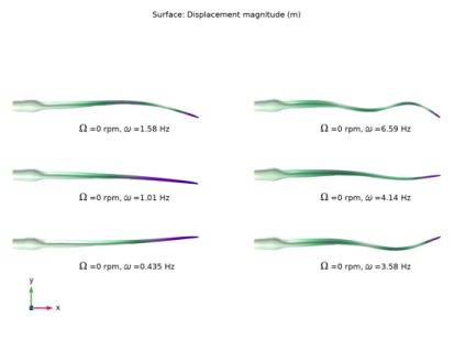
In the Model Builder window, expand the Results > Mode Shapes (shell) > Surface 1 node, then click Deformation.
2
In the Settings window for Deformation, locate the Scale section.
3
Select the Scale factor checkbox. In the associated text field, type 5e4.
Solution Array 1
1
In the Model Builder window, right-click Surface 1 and choose Solution Array.
2
In the Settings window for Solution Array, locate the Data section.
3
From the Parameter selection (RPM) list, choose Manual.
4
In the Parameter indices (1-7) text field, type 1.
5
From the Eigenfrequency selection list, choose Manual.
6
In the Eigenfrequency indices (1-8) text field, type range(1,1,6).
7
Locate the Plot Array section. From the Array shape list, choose Square.
8
From the Order list, choose Column-major.
Annotation 1
1
In the Model Builder window, right-click Mode Shapes (shell) and choose Annotation.
2
In the Settings window for Annotation, locate the Annotation section.
3
From the Geometry level list, choose Global.
4
In the Text text field, type $\Omega$ =eval(RPM, rpm, 3) rpm, $\omega$ =eval(freq, Hz, 3) Hz.
5
Select the LaTeX markup checkbox.
6
Locate the Position section. In the x text field, type 20.
7
In the y text field, type -5.
8
Locate the Coloring and Style section. Clear the Show point checkbox.
9
Click to expand the Plot Array section. Select the Manual indexing checkbox.
Solution Array 1
In the Model Builder window, under Results > Mode Shapes (shell) > Surface 1 right-click Solution Array 1 and choose Copy.
Solution Array 1
In the Model Builder window, right-click Annotation 1 and choose Paste Solution Array.
Mode Shapes (shell)
1
Click the  Go to XY View button in the Graphics toolbar.
2
Click the  Show Grid button in the Graphics toolbar.
3
In the Mode Shapes (shell) toolbar, click  Plot.
Campbell Diagram
1
In the Results toolbar, click  1D Plot Group.
2
In the Settings window for 1D Plot Group, type Campbell Diagram in the Label text field.
3
Locate the Data section. From the Dataset list, choose Study: Eigenfrequency/Parametric Solutions 1 (sol4).
4
Click to expand the Title section. From the Title type list, choose Label.
5
Locate the Plot Settings section.
6
Select the y-axis label checkbox. In the associated text field, type Frequency (Hz).
7
Locate the Legend section. Clear the Show legends checkbox.
Global 1
1
Right-click Campbell Diagram and choose Global.
2
In the Settings window for Global, locate the y-Axis Data section.
3
4
Locate the x-Axis Data section. From the Axis source data list, choose Outer solutions.
5
From the Parameter list, choose Expression.
6
In the Expression text field, type RPM.
7
In the Unit field, type rpm.
8
Click to expand the Coloring and Style section. Find the Line style subsection. From the Line list, choose Cycle.
9
Find the Line markers subsection. From the Marker list, choose Cycle.
10
In the Campbell Diagram toolbar, click  Plot.