|
|
|
|
|
|
G12
|
|
|
•
|
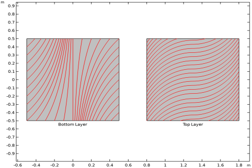
Modeling a composite laminate requires a surface geometry, referred to as the base surface, and a Layered Material node, which adds an extra dimension in the normal direction. You can use the Layered Material functionality to model several layers stacked on top of each other, each with a different thickness, material properties, and fiber orientation. You can optionally specify the interface materials between the layers and control the number of through-thickness mesh elements for each layer. To model a curvilinear fiber, add an expression as a function of the local coordinates in the Rotation field.
|
|
•
|
The third direction for the selected coordinate system in the Single Layer Material, Layered Material Link, or Layered Material Stack represents the normal direction. This is also the direction in which the layer stacking is interpreted from bottom to top, and therefore, it is crucial to visualize it during modeling. There are two ways to achieve this:
|
|
-
|
Using physics symbols: Go to the physics settings, find the Physics Symbols section, and select the Enable physics symbols checkbox. Then go to the material feature, for instance, Linear Elastic Material, to see the normal direction represented by green arrows.
|
|
-
|
Using result templates: When a solution dataset is available, use the result template Thickness and Orientation to plot the normal direction.
|
|
•
|
From a constitutive model viewpoint, you can either use the Layerwise (LW) theory available in the Layered Shell interface, or the Equivalent Single Layer (ESL) theory available in the Linear Elastic Material, Layered node in the Shell interface. The laminated composite presented in this example uses the Layered Shell interface.
|
|
•
|
The built-in Composites material library contains data for fiber and matrix constituents, as well as for unidirectional and bidirectional laminae.
|
|
1
|
|
2
|
|
3
|
Click Add.
|
|
4
|
|
5
|
Click Add.
|
|
6
|
Click
|
|
7
|
|
8
|
Click
|
|
1
|
|
2
|
|
3
|
Click
|
|
4
|
Browse to the model’s Application Libraries folder and double-click the file variable_angle_tow_laminate_parameters.txt.
|
|
1
|
|
2
|
|
3
|
|
4
|
|
5
|
|
6
|
|
7
|
|
8
|
Click to expand the Layers section. In the table, enter the following settings:
|
|
9
|
Click
|
|
1
|
Go to the Add Material window.
|
|
2
|
In the tree, select Composites > Laminae > Unidirectional fiber lamina: E-glass/epoxy [fiber volume fraction 60%].
|
|
3
|
Click the Add to Global Materials button in the window toolbar.
|
|
4
|
|
1
|
In the Model Builder window, under Global Definitions right-click Materials and choose Layered Material.
|
|
2
|
|
4
|
Click
|
|
1
|
|
2
|
|
3
|
|
4
|
|
6
|
|
7
|
|
1
|
|
2
|
|
3
|
|
4
|
Locate the Definition section. In the Expression text field, type 2/a*(thetae2-thetac2)*abs(x) + thetac2.
|
|
1
|
|
2
|
|
1
|
|
2
|
|
3
|
|
4
|
|
1
|
|
2
|
|
3
|
|
4
|
|
1
|
In the Model Builder window, under Component 1 (comp1) right-click Materials and choose Layers > Layered Material Link.
|
|
2
|
|
3
|
|
4
|
|
1
|
|
2
|
Click in the Graphics window and then press Ctrl+A to select both domains.
|
|
3
|
|
1
|
|
1
|
|
3
|
|
4
|
|
5
|
|
6
|
|
1
|
|
2
|
|
3
|
|
1
|
In the Model Builder window, under Component 1 (comp1) > Solid Mechanics (solid) click Linear Elastic Material 1.
|
|
2
|
|
3
|
|
4
|
Locate the Coordinate System Selection section. From the Coordinate system list, choose Rotated System (Solid, Bottom Layer) (sys2).
|
|
5
|
|
1
|
|
3
|
|
4
|
|
5
|
Locate the Coordinate System Selection section. From the Coordinate system list, choose Rotated System (Solid, Top Layer) (sys3).
|
|
6
|
|
1
|
|
1
|
|
3
|
|
4
|
|
5
|
|
1
|
|
1
|
|
3
|
|
4
|
|
1
|
|
2
|
|
3
|
|
4
|
Click
|
|
1
|
|
2
|
|
3
|
Click
|
|
4
|
|
5
|
|
6
|
Click OK.
|
|
7
|
|
9
|
Click
|
|
10
|
|
11
|
|
12
|
Click OK.
|
|
13
|
|
15
|
Select the Apply conversions to expressions with the same dimensions checkbox.
|
|
16
|
Click
|
|
1
|
|
2
|
|
3
|
Select the Show maximum and minimum values checkbox.
|
|
4
|
Select the Show units checkbox.
|
|
5
|
|
6
|
|
7
|
|
1
|
|
2
|
|
3
|
Select the Show maximum and minimum values checkbox.
|
|
4
|
Select the Show units checkbox.
|
|
1
|
|
2
|
|
3
|
|
4
|
|
1
|
|
2
|
|
3
|
|
4
|
|
5
|
|
6
|
|
7
|
|
8
|
|
1
|
|
2
|
|
3
|
|
4
|
|
1
|
|
2
|
|
3
|
Locate the Plot Settings section.
|
|
4
|
|
1
|
|
2
|
|
3
|
|
4
|
|
5
|
|
6
|
|
7
|
|
8
|
|
9
|
|
10
|
|
12
|
Select the Show legends checkbox.
|
|
1
|
|
2
|
|
3
|
|
4
|
|
5
|
|
6
|
|
7
|
Locate the Coloring and Style section. Find the Line style subsection. From the Line list, choose Dashed.
|
|
8
|
|
9
|
|
10
|
Locate the Legends section. In the table, enter the following settings:
|
|
11
|
|
1
|
|
2
|
|
3
|
|
4
|
|
1
|
|
2
|
|
3
|
|
1
|
|
2
|
|
3
|
|
1
|
|
2
|
|
1
|
In the Model Builder window, under Results, Ctrl-click to select u along Cut Line, v along Cut Line, w along Cut Line, sxx along Cut Line, sxy along Cut Line, sxz along Cut Line, syy along Cut Line, syz along Cut Line, szz along Cut Line, and von Mises along Cut Line.
|
|
2
|
Right-click and choose Group.
|
|
1
|
|
2
|
Go to the Result Templates window.
|
|
3
|
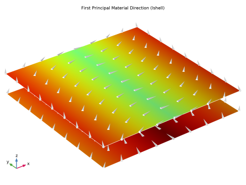
In the tree, select Study 1/Solution 1 (sol1) > Layered Shell > Geometry and Layup (lshell) > First Principal Material Direction (lshell).
|
|
4
|
Click the Add Result Template button in the window toolbar.
|
|
5
|
|
1
|
|
2
|
|
3
|
|
4
|
|
5
|
|
1
|
|
2
|
|
3
|
|
1
|
|
2
|
|
3
|
|
4
|
|
1
|
|
2
|
|
3
|
|
4
|
|
5
|
|
1
|
|
2
|
|
3
|
|
4
|
|
5
|
|
6
|
|
7
|
|
8
|
Locate the Coloring and Style section. Find the Point style subsection. From the Color list, choose Red.
|
|
9
|
|
1
|
|
2
|
|
3
|
|
1
|
|
2
|
|
3
|
|
4
|
|
1
|
|
2
|
|
3
|
|
4
|
|
1
|
In the Model Builder window, under Results > Fiber Path in Layers, Ctrl-click to select Surface 1, Streamline 1, and Streamline 2.
|
|
2
|
Right-click and choose Duplicate.
|
|
1
|
|
2
|
|
3
|
|
1
|
|
2
|
|
3
|
|
4
|
|
5
|
|
1
|
|
2
|
|
3
|
|
4
|
|
5
|
|
1
|
|
2
|
|
3
|
|
4
|
|
5
|
|
6
|
|
7
|
|
1
|
|
2
|
|
3
|
|
4
|
|
5
|