
|
|
|
 |
|
•
|
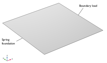
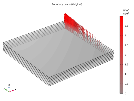
A total load of 12 kN, varying linearly with position, is applied to the right side of the laminate as a boundary load as shown in Figure 2.
 |
|
G12
|
|

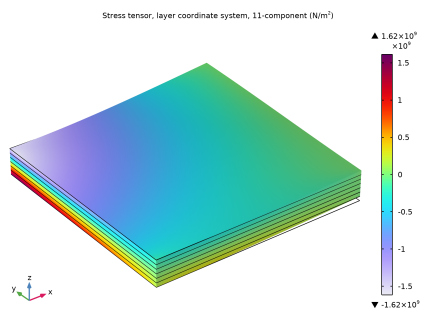
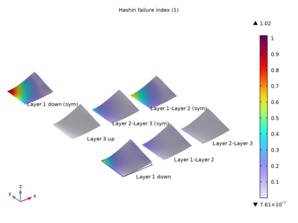
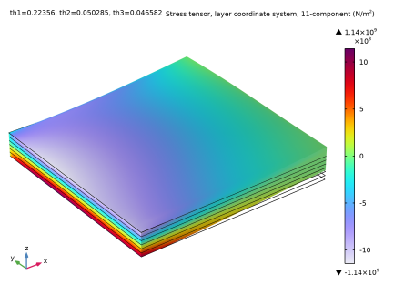
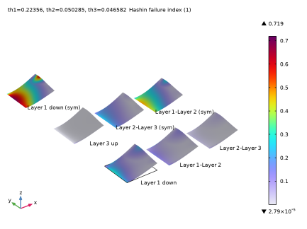
|
•
|
|
•
|
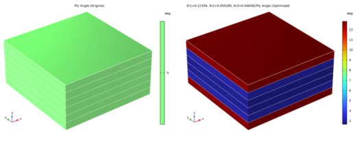
|
•
|
Modeling a composite laminate as a layered shell requires a surface geometry, in general referred to as a base surface, and a Layered Material node which adds an extra dimension (1D) to the base surface geometry in the surface normal direction. You can use the Layered Material functionality to model several layers stacked on top of each other having different thicknesses, material properties, and fiber orientations. You can optionally specify the interface materials between the layers, and control the number of through-thickness mesh elements for each layer.
|
|
•
|
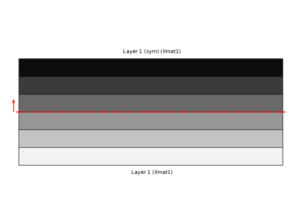
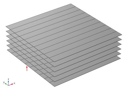
The third direction for the selected coordinate system in the Single Layer Material, Layered Material Link, or Layered Material Stack represents the normal direction of the Layered Shell or Shell physics. This is also the direction in which the layer stacking is interpreted from bottom to top, and therefore, it is crucial to know it during modeling. There are two ways to achieve this:
|
|
-
|
Using physics symbols: Go to the physics settings, find the Physics Symbols section, and select the Enable physics symbols checkbox. Then go to the material feature, for instance, Linear Elastic Material, to see the normal direction represented by green arrows in the geometry.
|
|
-
|
Using result templates: When a solution dataset is available, use the result template Thickness and Orientation to plot the normal direction.
|
|
•
|
From a constitutive model point of view, you can either use the Layerwise (LW) theory based Layered Shell interface, or the Equivalent Single Layer (ESL) theory based Linear Elastic Material, Layered node in the Shell interface. The laminated composite presented in the current model is modeled using the Layered Shell interface.
|
|
•
|
The built-in Composites material library contains data for fiber and matrix constituents as well as for unidirectional and bidirectional laminae.
|
|
1
|
|
2
|
|
3
|
Click Add.
|
|
4
|
Click
 Study. Study. |
|
5
|
|
6
|
Click
 Done. Done. |
|
1
|
|
2
|
|
3
|
Click
 Load from File. Load from File. |
|
4
|
Browse to the model’s Application Libraries folder and double-click the file stacking_sequence_optimization_parameters.txt.
|
|
1
|
|
2
|
Go to the Add Material window.
|
|
3
|
In the tree, select Composites > Laminae > Unidirectional fiber lamina: AS4/APC2 carbon/PEEK thermoplastic [fiber volume fraction 58%].
|
|
4
|
Right-click and choose Add to Global Materials.
|
|
5
|
|
1
|
In the Model Builder window, under Global Definitions right-click Materials and choose Layered Material.
|
|
2
|
|
4
|
Click Add two times.
|
|
6
|
|
1
|
|
2
|
|
1
|
|
2
|
|
3
|
|
4
|
|
5
|
|
6
|
|
7
|
|
1
|
In the Model Builder window, under Component 1 (comp1) right-click Materials and choose Layers > Layered Material Link.
|
|
2
|
|
3
|
|
4
|
Click to expand the Preview Plot Settings section. In the Thickness-to-width ratio text field, type 0.4.
|
|
5
|
Click Section_bar in the upper-right corner of the Layered Material Settings section. From the menu, choose Layer Cross-Section Preview.
|
|
6
|
Click Section_bar in the upper-right corner of the Layered Material Settings section. From the menu, choose Layer Stack Preview.
|
|
1
|
|
2
|
|
3
|
|
1
|
|
3
|
|
4
|
|
5
|
From the list, choose Diagonal.
|
|
6
|
|
1
|
|
3
|
|
4
|
|
5
|
|
1
|
|
2
|
|
3
|
|
4
|
|
1
|
|
2
|
|
3
|
Click
 Load from File. Load from File. |
|
4
|
Browse to the model’s Application Libraries folder and double-click the file stacking_sequence_optimization_variables.txt.
|
|
1
|
|
1
|
|
3
|
|
4
|
|
5
|
|
6
|
|
7
|
|
1
|
|
3
|
|
4
|
|
5
|
|
6
|
|
7
|
|
8
|
Select the Symmetric distribution checkbox.
|
|
9
|
Click
 Build All. Build All. |
|
1
|
|
2
|
|
3
|
|
1
|
|
2
|
In the Settings window for Evaluation Group, type Failure Indices and Fiber Orientations (Original) in the Label text field.
|
|
3
|
|
4
|
|
5
|
|
1
|
|
2
|
|
4
|
|
1
|
|
2
|
|
3
|
|
1
|
|
2
|
In the Settings window for 3D Plot Group, type Stress, Layer Coordinate System (Original) in the Label text field.
|
|
3
|
|
4
|
|
1
|
|
2
|
Go to the Result Templates window.
|
|
3
|
In the tree, select Study 1: Original Layup/Solution 1 (sol1) > Layered Shell > Stress, Slice (lshell).
|
|
4
|
Click the Add Result Template button in the window toolbar.
|
|
1
|
In the Settings window for 3D Plot Group, type Failure Index, Slice (Original) in the Label text field.
|
|
2
|
|
1
|
In the Model Builder window, expand the Failure Index, Slice (Original) node, then click Layered Material Slice 1.
|
|
2
|
In the Settings window for Layered Material Slice, click Replace Expression in the upper-right corner of the Expression section. From the menu, choose Component 1 (comp1) > Layered Shell > Safety > Hashin > lshell.lemm1.sf1.f_i - Hashin failure index - 1.
|
|
3
|
Locate the Through-Thickness Location section. From the Location definition list, choose Interfaces.
|
|
4
|
|
5
|
|
6
|
|
7
|
Select the Show descriptions checkbox.
|
|
8
|
|
9
|
|
10
|
|
11
|
|
12
|
|
1
|
|
2
|
|
3
|
|
4
|
|
5
|
|
1
|
Go to the Result Templates window.
|
|
2
|
In the tree, select Study 1: Original Layup/Solution 1 (sol1) > Layered Shell > Geometry and Layup (lshell) > Ply Angle (lshell).
|
|
3
|
Click the Add Result Template button in the window toolbar.
|
|
1
|
|
2
|
Click
 Go to Source. Go to Source. |
|
1
|
|
2
|
|
3
|
|
1
|
|
2
|
|
3
|
Clear the Manual color range checkbox.
|
|
1
|
|
2
|
|
3
|
|
4
|
|
1
|
Go to the Result Templates window.
|
|
2
|
In the tree, select Study 1: Original Layup/Solution 1 (sol1) > Layered Shell > Applied Loads (lshell) > Boundary Loads (lshell).
|
|
3
|
Click the Add Result Template button in the window toolbar.
|
|
1
|
|
2
|
|
1
|
In the Model Builder window, expand the Results > Boundary Loads (Original) > Boundary Load 1 node, then click Boundary Load 1.
|
|
2
|
|
3
|
|
4
|
|
1
|
|
2
|
Go to the Add Study window.
|
|
3
|
|
4
|
Click the Add Study button in the window toolbar.
|
|
5
|
|
1
|
|
2
|
|
3
|
|
4
|
|
5
|
Locate the Objective Function section. In the table, enter the following settings:
|
|
6
|
|
8
|
|
1
|
|
2
|
|
3
|
|
1
|
|
2
|
In the Settings window for 3D Plot Group, type Stress, Layer Coordinate System (Optimized) in the Label text field.
|
|
3
|
|
4
|
|
1
|
Go to the Result Templates window.
|
|
2
|
In the tree, select Study 2: Layup Optimization/Parametric Solutions 1 (sol3) > Layered Shell > Stress, Slice (lshell).
|
|
3
|
Click the Add Result Template button in the window toolbar.
|
|
1
|
In the Settings window for 3D Plot Group, type Failure Index, Slice (Optimized) in the Label text field.
|
|
2
|
|
1
|
In the Model Builder window, expand the Failure Index, Slice (Optimized) node, then click Layered Material Slice 1.
|
|
2
|
In the Settings window for Layered Material Slice, click Replace Expression in the upper-right corner of the Expression section. From the menu, choose Component 1 (comp1) > Layered Shell > Safety > Hashin > lshell.lemm1.sf1.f_i - Hashin failure index - 1.
|
|
3
|
Locate the Through-Thickness Location section. From the Location definition list, choose Interfaces.
|
|
4
|
|
5
|
|
6
|
|
7
|
Select the Show descriptions checkbox.
|
|
8
|
|
9
|
|
10
|
|
1
|
|
2
|
|
3
|
|
4
|
|
1
|
Go to the Result Templates window.
|
|
2
|
In the tree, select Study 2: Layup Optimization/Parametric Solutions 1 (sol3) > Layered Shell > Geometry and Layup (lshell) > Ply Angle (lshell).
|
|
3
|
Click the Add Result Template button in the window toolbar.
|
|
4
|
|
1
|
|
2
|
Click
 Go to Source. Go to Source. |
|
1
|
|
2
|
|
3
|
|
1
|
|
2
|
|
3
|
Clear the Manual color range checkbox.
|
|
1
|
|
2
|
|
3
|
|
4
|
|
1
|
|
2
|
|
3
|
Clear the Plot dataset edges checkbox.
|
|
1
|
In the Model Builder window, expand the Failure Index, Slice (Original) 1 node, then click Layered Material Slice 1.
|
|
2
|
|
3
|
|
4
|
|
5
|
Locate the Through-Thickness Location section. From the Location definition list, choose Reference surface.
|
|
6
|
|
7
|
Clear the Show descriptions checkbox.
|
|
8
|
|
9
|
Select the Wireframe checkbox.
|
|
1
|
In the Model Builder window, expand the Results > Failure Index, Slice (Original) 1 > Layered Material Slice 1 node, then click Deformation.
|
|
2
|
|
3
|
|
1
|
|
2
|
|
3
|
|
1
|
In the Model Builder window, under Results > Failure Index, Slice (Original) 1 click Layered Material Slice 2.
|
|
2
|
|
3
|
|
4
|
|
5
|
|
6
|
|
1
|
|
2
|
|
3
|
|
4
|
Locate the Expression section. In the Expression text field, type lshell.atxd1(lshell.d/2,mean(lshell.disp)).
|
|
5
|
|
6
|
|
7
|
|
8
|
|
9
|
|
1
|
|
2
|
|
3
|
|
4
|
|
5
|
|
1
|
|
2
|
|
3
|
|
1
|
|
2
|
|
3
|
|
1
|
|
2
|
In the Settings window for 3D Plot Group, type Displacement: Original and Optimized in the Label text field.
|
|
3
|
|
4
|
|
5
|
|
1
|
In the Model Builder window, right-click Failure Indices and Fiber Orientations (Original) and choose Duplicate.
|
|
2
|
In the Settings window for Evaluation Group, type Failure Indices and Fiber Orientations (Optimized) in the Label text field.
|
|
3
|
|
4
|
|
5
|


