|
|
|
|
|
|
G12
|
|
|
•
|
Modeling a composite laminate as a layered shell requires a surface geometry, referred to as a the base surface, and a Layered Material node, which adds an extra dimension (1D) in the normal direction. You can use the Layered Material functionality to model several layers stacked on top of each other, each having a different thickness, material properties, and fiber orientation. You can optionally specify the interface material between the layers and control the number of through-thickness mesh elements for each layer. To model a curvilinear fiber, add an expression as a function of the local coordinates in the Rotation field.
|
|
•
|
The third direction for the selected coordinate system in the Single Layer Material, Layered Material Link, or Layered Material Stack represents the normal direction. This is also the direction in which the layer stacking is interpreted from bottom to top, and therefore, it is crucial to visualize it during modeling. There are two ways to achieve this:
|
|
-
|
Using physics symbols: Go to the physics settings, find the Physics Symbols section, and select the Enable physics symbols checkbox. Then go to the material feature, for instance, Linear Elastic Material, to see the normal direction represented by green arrows.
|
|
-
|
Using result templates: When a solution dataset is available, use the result template Thickness and Orientation to plot the normal direction.
|
|
•
|
From a constitutive model point of view, you can either use the Layerwise (LW) theory available in the Layered Shell interface, or the Equivalent Single Layer (ESL) theory available in the Linear Elastic Material, Layered node in the Shell interface. The laminated composite presented in this example uses the Layered Shell interface.
|
|
•
|
The built-in Composites material library contains data for fiber and matrix constituents as well as for unidirectional and bidirectional laminae.
|
|
1
|
|
2
|
|
3
|
Click Add.
|
|
4
|
Click
|
|
5
|
|
6
|
Click
|
|
1
|
|
2
|
|
3
|
Click
|
|
4
|
Browse to the model’s Application Libraries folder and double-click the file fiber_angle_optimization_parameters.txt.
|
|
1
|
|
2
|
|
4
|
|
5
|
Locate the Variables section. In the table, enter the following settings:
|
|
1
|
|
2
|
Go to the Add Material window.
|
|
3
|
In the tree, select Composites > Laminae > Unidirectional fiber lamina: AS4/APC2 carbon/PEEK thermoplastic [fiber volume fraction 58%].
|
|
4
|
Right-click and choose Add to Global Materials.
|
|
5
|
|
1
|
In the Model Builder window, under Global Definitions right-click Materials and choose Layered Material.
|
|
2
|
|
1
|
|
2
|
|
3
|
|
1
|
|
2
|
|
3
|
|
1
|
|
2
|
Select the object sq1 only.
|
|
3
|
|
4
|
|
5
|
Select the object c1 only.
|
|
6
|
|
7
|
|
1
|
In the Model Builder window, under Component 1 (comp1) right-click Materials and choose Layers > Layered Material Link.
|
|
2
|
|
3
|
|
1
|
In the Model Builder window, under Component 1 (comp1) > Definitions click Boundary System 1 (sys1).
|
|
2
|
|
3
|
|
1
|
|
2
|
|
3
|
|
1
|
|
1
|
|
3
|
|
4
|
|
1
|
|
3
|
|
4
|
|
1
|
|
3
|
|
1
|
|
2
|
|
3
|
|
4
|
Click
|
|
1
|
|
2
|
|
3
|
|
1
|
|
2
|
|
1
|
|
2
|
|
3
|
Click
|
|
5
|
|
1
|
|
2
|
|
3
|
Click
|
|
4
|
|
5
|
Click OK.
|
|
6
|
|
8
|
Click
|
|
9
|
|
10
|
Click OK.
|
|
11
|
|
13
|
Select the Apply conversions to expressions with the same dimensions checkbox.
|
|
14
|
Click
|
|
1
|
|
2
|
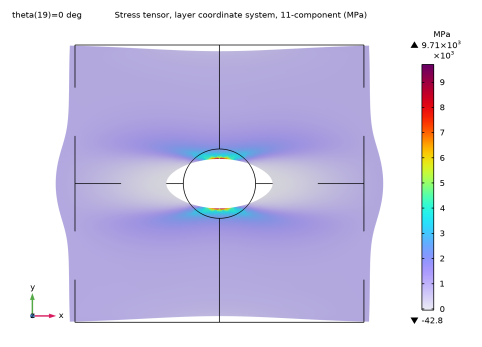
In the Settings window for Layered Material, type Layered Material (Original Orientation) in the Label text field.
|
|
1
|
|
2
|
|
3
|
|
1
|
|
2
|
In the Settings window for Mirror 3D, type Mirror 3D (Original Orientation) in the Label text field.
|
|
3
|
|
4
|
|
1
|
|
2
|
In the Settings window for 3D Plot Group, type Stress (Original Orientation) in the Label text field.
|
|
3
|
|
4
|
|
5
|
|
6
|
Select the Show units checkbox.
|
|
7
|
|
1
|
|
2
|
|
3
|
|
4
|
|
5
|
|
6
|
Locate the Control Variable Discretization section. From the Control type list, choose Piecewise Bernstein polynomial.
|
|
7
|
|
8
|
|
9
|
|
10
|
Click OK.
|
|
1
|
|
2
|
|
3
|
|
1
|
|
2
|
|
4
|
|
1
|
|
2
|
|
3
|
Select the Modify model configuration for study step checkbox.
|
|
4
|
|
5
|
Click
|
|
1
|
|
2
|
Go to the Add Study window.
|
|
3
|
|
4
|
Click the Add Study button in the window toolbar.
|
|
5
|
|
1
|
|
2
|
|
3
|
|
4
|
Locate the Objective Function section. In the table, enter the following settings:
|
|
1
|
|
2
|
|
3
|
Select the Modify model configuration for study step checkbox.
|
|
4
|
|
5
|
Click
|
|
6
|
|
1
|
|
2
|
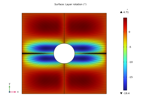
In the Settings window for Layered Material, type Layered Material (Optimization) in the Label text field.
|
|
1
|
|
2
|
|
3
|
|
1
|
|
2
|
In the Settings window for Mirror 3D, type Mirror 3D (Optimized Orientation) in the Label text field.
|
|
3
|
|
1
|
|
2
|
In the Settings window for 3D Plot Group, type Stress (Optimized Orientation) in the Label text field.
|
|
3
|
|
4
|
|
5
|
Select the Show units checkbox.
|
|
6
|
|
1
|
|
2
|
|
3
|
|
4
|
|
5
|
|
6
|
|
7
|
|
1
|
|
2
|
|
3
|
|
4
|
|
5
|
|
1
|
|
2
|
|
3
|
|
4
|
|
5
|
|
6
|
|
7
|
|
8
|
|
9
|
Locate the Coloring and Style section. Find the Point style subsection. From the Color list, choose Black.
|
|
10
|
|
11
|
Select the Radius scale factor checkbox.
|
|
12
|
|
1
|
|
2
|
|
3
|
|
1
|
|
2
|
|
3
|
|
4
|
|
5
|
|
6
|
|
7
|
Locate the Coloring and Style section.
|
|
8
|
|
9
|
|
1
|
|
2
|
|
3
|
|
1
|
|
2
|
|
3
|
|
4
|
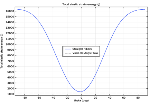
Locate the y-Axis Data section. In the table, enter the following settings:
|
|
5
|
|
1
|
|
2
|
|
3
|
|
4
|
Locate the x-Coordinates section. In the table, enter the following settings:
|
|
5
|
Locate the y-Coordinates section. In the table, enter the following settings:
|
|
6
|
Click to expand the Coloring and Style section. Find the Line style subsection. From the Line list, choose Dashed.
|
|
7
|
|
8
|
|
9
|
|
11
|
|
1
|
|
2
|
|
3
|
|
4
|
Locate the Plot Settings section.
|
|
5
|
|
1
|
|
2
|
|
1
|
|
2
|
|
4
|