|
|
|
|
|
|
•
|
|
•
|
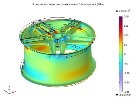
Stationary analysis: This analysis is performed for the tire pressure and total load on the wheels. The overpressure is 2 bar = 200 kPa. The total load carried by the wheel corresponds to a weight of 1120 kg. It is applied as a pressure on the rim surfaces where the tire is in contact. Assume that the load distribution in the circumferential direction can be approximated as p = p0 cos ( 3 ϑ ), where ϑ is the angle from the point of contact between the road and the tire. The loaded area thus extends 30° in each direction from the load peak.
|
|
•
|
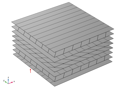
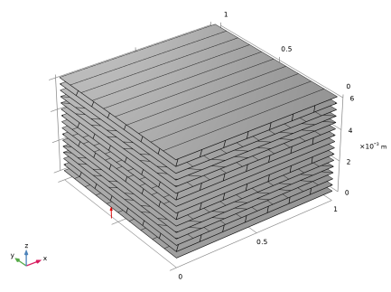
Modeling a composite laminate as a layered shell requires a surface geometry, in general referred to as a base surface, and a Layered Material node which adds an extra dimension (1D) to the base surface geometry in the surface normal direction. You can use the Layered Material functionality to model several layers stacked on top of each other having different thicknesses, material properties, and fiber orientations. You can optionally specify the interface materials between the layers, and control the number of through-thickness mesh elements for each layer.
|
|
•
|
The third direction for the selected coordinate system in the Single Layer Material, Layered Material Link, or Layered Material Stack represents the normal direction of the Layered Shell or Shell physics. This is also the direction in which the layer stacking is interpreted from bottom to top, and therefore, it is crucial to know it during modeling. There are two ways to achieve this:
|
|
-
|
Using physics symbols: Go to the physics settings, find the Physics Symbols section, and select the Enable physics symbols checkbox. Then go to the material feature, for instance, Linear Elastic Material, to see the normal direction represented by green arrows in the geometry.
|
|
-
|
Using result templates: When a solution dataset is available, use the result template Thickness and Orientation to plot the normal direction.
|
|
•
|
From a constitutive model point of view, you can either use the Layerwise (LW) theory based Layered Shell interface, or the Equivalent Single Layer (ESL) theory based Linear Elastic Material, Layered node in the Shell interface. The laminated composite shell presented in the current model is modeled using a Linear Elastic Material, Layered node in the Shell interface.
|
|
•
|
The built-in Composites material library contains data for fiber and matrix constituents as well as for unidirectional and bidirectional laminae.
|
|
1
|
|
2
|
|
3
|
Click Add.
|
|
4
|
Click
|
|
5
|
|
6
|
Click
|
|
1
|
|
2
|
|
3
|
Click
|
|
4
|
Browse to the model’s Application Libraries folder and double-click the file composite_wheel_rim_parameters.txt.
|
|
1
|
|
2
|
|
3
|
|
4
|
Locate the Definition section. In the Expression text field, type (abs(atan2(x,y)-z*pi/180)<pi/6)*cos(3*(atan2(x,y)-z*pi/180)).
|
|
5
|
|
6
|
Locate the Units section. In the table, enter the following settings:
|
|
7
|
|
1
|
|
2
|
|
3
|
|
4
|
|
5
|
Click
|
|
6
|
Browse to the model’s Application Libraries folder and double-click the file composite_wheel_rim.mphbin.
|
|
7
|
Click
|
|
8
|
Click
|
|
1
|
|
2
|
|
3
|
|
4
|
On the object imp1, select Boundaries 11–19, 24, 26, 28, and 34–36 only.
|
|
1
|
|
2
|
|
3
|
|
4
|
|
5
|
|
6
|
Click OK.
|
|
1
|
|
2
|
|
3
|
|
4
|
On the object imp1, select Boundaries 16–19, 24, 26, 35, and 36 only.
|
|
1
|
|
2
|
|
3
|
|
4
|
|
5
|
On the object imp1, select Boundaries 8 and 30 only.
|
|
1
|
|
2
|
Select the object imp1 only.
|
|
3
|
|
4
|
|
5
|
Click
|
|
1
|
|
2
|
|
3
|
|
4
|
|
5
|
|
6
|
|
7
|
|
8
|
|
9
|
|
10
|
Clear the Automatic detection of small details checkbox.
|
|
11
|
|
1
|
|
2
|
|
3
|
|
4
|
|
5
|
|
1
|
|
2
|
Go to the Add Material window.
|
|
3
|
In the tree, select Composites > Laminae > Unidirectional fiber lamina: AS4/APC2 carbon/PEEK thermoplastic [fiber volume fraction 58%].
|
|
4
|
Right-click and choose Add to Global Materials.
|
|
5
|
|
1
|
In the Model Builder window, under Global Definitions right-click Materials and choose Layered Material.
|
|
2
|
|
4
|
Click Add three times.
|
|
1
|
In the Model Builder window, under Component 1 (comp1) right-click Materials and choose Layers > Layered Material Link.
|
|
2
|
|
3
|
|
4
|
|
5
|
|
6
|
Click to expand the Preview Plot Settings section. In the Thickness-to-width ratio text field, type 0.6.
|
|
7
|
Locate the Layered Material Settings section. Click Layer Stack Preview in the upper-right corner of the section.
|
|
1
|
|
2
|
|
3
|
|
4
|
|
5
|
|
6
|
|
1
|
|
2
|
|
3
|
|
1
|
|
2
|
In the Settings window for Layered Material Stack, click to expand the Preview Plot Settings section.
|
|
3
|
|
4
|
Locate the Layered Material Settings section. Click Layer Stack Preview in the upper-right corner of the section.
|
|
1
|
|
2
|
|
3
|
|
4
|
|
1
|
|
2
|
|
3
|
|
1
|
|
2
|
|
3
|
|
4
|
|
5
|
|
6
|
|
1
|
|
2
|
|
3
|
|
4
|
Locate the Coordinate System Selection section. From the Coordinate system list, choose Cylindrical System 2 (sys2).
|
|
5
|
|
6
|
|
7
|
|
8
|
|
9
|
|
10
|
Click OK.
|
|
1
|
|
2
|
|
4
|
|
5
|
|
6
|
|
7
|
Click OK.
|
|
1
|
|
2
|
|
3
|
|
1
|
|
2
|
|
3
|
From the list, choose User-controlled mesh.
|
|
1
|
|
2
|
|
3
|
|
4
|
|
5
|
|
6
|
Click
|
|
1
|
|
2
|
|
1
|
|
2
|
|
3
|
Select the Modify model configuration for study step checkbox.
|
|
4
|
|
5
|
Click
|
|
6
|
|
1
|
|
2
|
|
3
|
Click
|
|
4
|
|
5
|
Click OK.
|
|
6
|
|
8
|
Click
|
|
1
|
|
2
|
|
3
|
|
4
|
|
5
|
|
6
|
|
1
|
|
2
|
|
3
|
Select the Show maximum and minimum values checkbox.
|
|
4
|
|
1
|
|
2
|
Go to the Result Templates window.
|
|
3
|
|
4
|
Click the Add Result Template button in the window toolbar.
|
|
5
|
|
6
|
Click the Add Result Template button in the window toolbar.
|
|
7
|
|
1
|
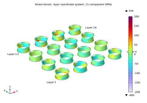
In the Model Builder window, expand the Results > Stress, Slice (shell) node, then click Layered Material Slice 1.
|
|
2
|
|
3
|
Select the Manual color range checkbox.
|
|
4
|
|
5
|
|
1
|
|
2
|
|
3
|
Select the Show maximum and minimum values checkbox.
|
|
4
|
|
1
|
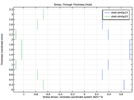
In the Model Builder window, expand the Results > Stress, Through Thickness (shell) node, then click Through Thickness 1.
|
|
2
|
|
3
|
Click to select the
|
|
4
|
Click
|
|
6
|
|
1
|
|
2
|
|
3
|
Click to select the
|
|
4
|
Click
|
|
6
|
|
1
|
|
2
|
In the Settings window for 1D Plot Group, type Stress, Through Thickness [Rim] in the Label text field.
|
|
3
|
|
1
|
In the Model Builder window, expand the Stress, Through Thickness [Rim] 1 node, then click Through Thickness 1.
|
|
2
|
|
3
|
Click to select the
|
|
4
|
Click
|
|
1
|
|
2
|
|
3
|
Click to select the
|
|
4
|
Click
|
|
1
|
|
2
|
In the Settings window for 1D Plot Group, type Stress, Through Thickness [Hub] in the Label text field.
|
|
3
|
|
1
|
|
2
|
In the Settings window for 3D Plot Group, type Stress, Slice (Hub and Spokes) in the Label text field.
|
|
3
|
|
4
|
|
5
|
Select the Apply to dataset edges checkbox.
|
|
6
|
|
1
|
In the Model Builder window, expand the Stress, Slice (Hub and Spokes) node, then click Layered Material Slice 1.
|
|
2
|
|
3
|
|
4
|
|
5
|
|
6
|
Select the Show descriptions checkbox.
|
|
7
|
|
1
|
|
2
|
|
3
|
|
1
|
|
2
|
|
3
|
Clear the Plot dataset edges checkbox.
|
|
4
|
|
1
|
|
2
|
|
3
|
|
4
|
|
5
|
|
1
|
In the Model Builder window, expand the Stress, Slice (Rim) node, then click Layered Material Slice 1.
|
|
2
|
|
3
|
|
4
|
|
5
|
Clear the Show descriptions checkbox.
|
|
1
|
In the Model Builder window, right-click Stress, Slice (Rim) and choose More Plots > Table Annotation.
|
|
2
|
|
3
|
|
5
|
|
1
|
|
2
|
|
1
|
|
2
|
Go to the Add Study window.
|
|
3
|
|
4
|
Click the Add Study button in the window toolbar.
|
|
5
|
|
1
|
|
2
|
|
3
|
Select the Modify model configuration for study step checkbox.
|
|
4
|
In the tree, select Component 1 (comp1) > Shell (shell) > Face Load 1, Component 1 (comp1) > Shell (shell) > Face Load 2, and Component 1 (comp1) > Shell (shell) > Global Equations 1 (ODE1).
|
|
5
|
Click
|
|
1
|
|
2
|
|
3
|
Select the Include geometric nonlinearity checkbox.
|
|
4
|
|
1
|
|
2
|
|
3
|
Clear the Parameter indicator text field.
|
|
4
|
|
5
|
|
6
|
|
1
|
|
2
|
|
3
|
|
4
|
|
5
|
|
6
|
|
1
|
|
2
|
|
3
|
|
4
|
|
5
|
|
6
|
|
7
|
|
8
|
|
1
|
|
2
|
|
3
|
|
4
|
|
5
|
|
1
|
|
2
|
Go to the Result Templates window.
|
|
3
|
|
4
|
Click the Add Result Template button in the window toolbar.
|
|
5
|
|
1
|
|
2
|
|
3
|