
|
|
|
|
|
|
{230,15} GPa
|
|
|
G12
|
27 GPa
|
|
•
|
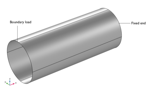
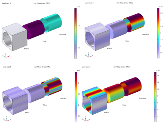
The other end has a transverse load of 75 kN, represented as a uniform boundary load on cross section.
|

|
•
|
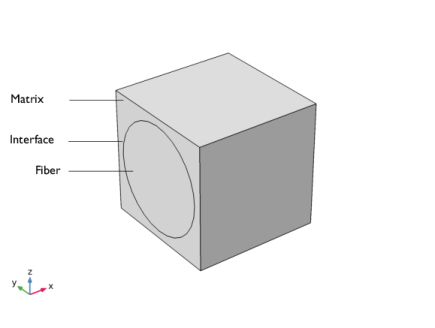
Modeling a composite laminated shell requires a 2D surface geometry, called a base surface, and a Layered Material node that adds an extra dimension (1D) to the base surface geometry in the surface normal direction. Using the Layered Material functionality, you can model several layers of different thicknesses, material properties, and fiber orientations. You can optionally specify the interface materials between the layers and the control mesh elements in each layer.
|
|
•
|
The Layered Material Link and Layered Material Stack have an option to transform the given Layered Material into a symmetric or antisymmetric laminate. A repeated laminate can also be constructed using a transform option.
|
|
•
|
The third direction for the selected coordinate system in the Single Layer Material, Layered Material Link, or Layered Material Stack represents the normal direction of the Layered Shell or Shell physics. This is also the direction in which the layer stacking is interpreted from bottom to top, and therefore, it is crucial to know it during modeling. There are two ways to achieve this:
|
|
-
|
Using physics symbols: Go to the physics settings, find the Physics Symbols section, and select the Enable physics symbols checkbox. Then go to the material feature, for instance, Linear Elastic Material, to see the normal direction represented by green arrows in the geometry.
|
|
-
|
Using result templates: When a solution dataset is available, use the result template Thickness and Orientation to plot the normal direction.
|
|
•
|
The built-in Composites material library contains data for fiber and matrix constituents as well as for unidirectional and bidirectional laminae.
|
|
•
|
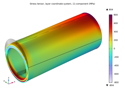
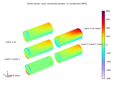
To analyze the results in a composite shell, you can either create a slice plot using the Layered Material Slice plot for in-plane variation of a quantity, or you can create a Through Thickness plot for out-of-plane variation of a quantity at a point. To visualize the results as a 3D solid object, you can use the Layered Material dataset, which creates a virtual 3D solid object combining the surface geometry (2D) and the extra dimension (1D).
|
|
1
|
|
2
|
|
3
|
Click Add.
|
|
4
|
Click
|
|
1
|
|
2
|
|
3
|
|
4
|
Browse to the model’s Application Libraries folder and double-click the file composite_multiscale_parameters.txt.
|
|
1
|
|
2
|
|
3
|
|
4
|
Browse to the model’s Application Libraries folder and double-click the file composite_multiscale_material_properties.txt.
|
|
1
|
|
2
|
|
3
|
|
4
|
Browse to the model’s Application Libraries folder and double-click the file composite_multiscale_strength_properties.txt.
|
|
5
|
In the Model Builder window, right-click Global Definitions and choose Geometry Parts > Part Libraries.
|
|
1
|
In the Part Libraries window, select COMSOL Multiphysics > Unit Cells and RVEs > Fiber Composites > unidirectional_fiber_square_packing in the tree.
|
|
2
|
Click
|
|
3
|
|
4
|
Click OK.
|
|
1
|
|
2
|
In the Settings window for Component, type Component: Micromechanics (Material Properties) in the Label text field.
|
|
1
|
In the Geometry toolbar, click
|
|
2
|
|
4
|
Locate the Position and Orientation of Output section. Find the Displacement subsection. In the xwi text field, type -0.005[m].
|
|
5
|
|
6
|
|
1
|
|
2
|
|
3
|
|
1
|
|
2
|
|
3
|
|
4
|
On the object fin, select Boundaries 6–9 only.
|
|
5
|
|
1
|
In the Model Builder window, under Component: Micromechanics (Material Properties) (comp1) > Solid Mechanics (solid) click Linear Elastic Material 1.
|
|
2
|
|
3
|
|
1
|
|
2
|
|
3
|
|
4
|
|
1
|
|
2
|
|
3
|
|
4
|
|
5
|
Select the Compute elasticity matrix, standard notation checkbox.
|
|
1
|
|
2
|
|
3
|
|
1
|
|
2
|
|
3
|
|
1
|
|
2
|
|
3
|
|
1
|
|
2
|
In the Settings window for Cell Periodicity, click Automated Model Setup in the upper-right corner of the Periodicity Settings section. From the menu, choose Create Load Groups and Study to generate load groups and a study node.
|
|
1
|
In the Model Builder window, under Component: Micromechanics (Material Properties) (comp1) right-click Materials and choose More Materials > Material Link.
|
|
2
|
|
3
|
Locate the Geometric Entity Selection section. From the Selection list, choose Matrix (Unidirectional Fiber Composite, Square Packing 1).
|
|
4
|
|
1
|
Go to the Add Material to Material Link 1: Matrix (matlnk1) window.
|
|
2
|
|
3
|
Click Add Material.
|
|
1
|
|
2
|
|
3
|
Locate the Geometric Entity Selection section. From the Selection list, choose Fiber (Unidirectional Fiber Composite, Square Packing 1).
|
|
4
|
|
1
|
Go to the Add Material to Material Link 2: Fiber (matlnk2) window.
|
|
2
|
|
3
|
Click Add Material.
|
|
1
|
|
2
|
|
3
|
Locate the Geometric Entity Selection section. From the Geometric entity level list, choose Boundary.
|
|
4
|
|
5
|
|
1
|
|
2
|
|
3
|
Locate the Material Contents section. In the table, enter the following settings:
|
|
1
|
|
2
|
|
3
|
|
4
|
Locate the Second Entity Group section. From the Selection list, choose Pair 1, Destination (Unidirectional Fiber Composite, Square Packing 1).
|
|
1
|
|
2
|
|
3
|
|
4
|
Click
|
|
1
|
|
2
|
|
1
|
|
2
|
In the Settings window for Study, type Study: Micromechanics (Material Properties) in the Label text field.
|
|
3
|
|
1
|
|
2
|
|
3
|
Click
|
|
4
|
|
5
|
Click OK.
|
|
6
|
|
8
|
Click
|
|
1
|
|
2
|
|
3
|
|
4
|
|
1
|
|
2
|
|
1
|
In the Model Builder window, under Results > Stress, Unit Cell right-click Volume 1 and choose Duplicate.
|
|
2
|
|
3
|
|
4
|
|
1
|
|
2
|
|
3
|
Click
|
|
1
|
|
2
|
|
3
|
|
4
|
|
1
|
|
2
|
|
1
|
|
2
|
|
3
|
|
5
|
|
1
|
|
2
|
|
3
|
|
4
|
|
1
|
In the Model Builder window, under Component: Micromechanics (Material Properties) (comp1) > Solid Mechanics (solid) click Cell Periodicity 1.
|
|
2
|
In the Settings window for Cell Periodicity, click Automated Model Setup in the upper-right corner of the Periodicity Settings section. From the menu, choose Create Material by Value to generate a global material node with computed elastic properties.
|
|
1
|
|
2
|
|
3
|
|
4
|
|
5
|
|
6
|
|
7
|
Click
|
|
8
|
|
1
|
In the Model Builder window, expand the Component: Macromechanics (Global Response) (comp2) > Definitions node, then click Boundary System 2 (sys2).
|
|
2
|
|
3
|
|
1
|
|
2
|
Go to the Add Physics window.
|
|
3
|
|
4
|
Find the Physics interfaces in study subsection. In the table, clear the Solve checkbox for Study: Micromechanics (Material Properties).
|
|
5
|
Click the Add to Component: Macromechanics (Global Response) button in the window toolbar.
|
|
6
|
|
1
|
In the Model Builder window, under Global Definitions right-click Materials and choose Layered Material.
|
|
2
|
In the Settings window for Layered Material, type Layered Material: [90/0]_2 in the Label text field.
|
|
3
|
Locate the Layer Definition section. In the table, enter the following settings:
|
|
4
|
Click Add.
|
|
1
|
In the Model Builder window, under Component: Macromechanics (Global Response) (comp2) right-click Materials and choose Layers > Layered Material Link.
|
|
2
|
|
3
|
|
4
|
|
5
|
Click to expand the Preview Plot Settings section. In the Thickness-to-width ratio text field, type 0.4.
|
|
6
|
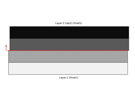
Locate the Layered Material Settings section. Click Layer Cross-Section Preview in the upper-right corner of the section to enable the through-thickness view of the laminated material.
|
|
7
|
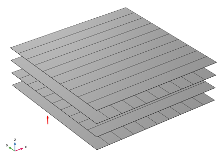
Click Layer Stack Preview in the upper-right corner of the Layered Material Settings section to show the stacking sequence including the fiber orientation.
|
|
1
|
In the Model Builder window, under Component: Macromechanics (Global Response) (comp2) > Layered Shell (lshell) click Linear Elastic Material 1.
|
|
2
|
|
3
|
|
1
|
|
2
|
|
3
|
|
1
|
|
2
|
|
3
|
|
4
|
|
5
|
|
1
|
In the Model Builder window, under Global Definitions > Materials click Homogeneous Material (solidcp1mat).
|
|
2
|
|
1
|
|
1
|
|
3
|
|
4
|
|
5
|
|
1
|
|
2
|
|
3
|
|
1
|
|
2
|
|
3
|
|
4
|
|
5
|
Click
|
|
1
|
|
2
|
Go to the Add Study window.
|
|
3
|
|
4
|
Find the Physics interfaces in study subsection. In the table, clear the Solve checkbox for Solid Mechanics (solid).
|
|
5
|
Click the Add Study button in the window toolbar.
|
|
6
|
|
1
|
In the Settings window for Study, type Study: Macromechanics (Global Response) in the Label text field.
|
|
2
|
|
1
|
|
2
|
|
3
|
|
1
|
|
2
|
|
3
|
|
4
|
|
1
|
|
2
|
|
1
|
|
2
|
Go to the Result Templates window.
|
|
3
|
In the tree, select Study: Macromechanics (Global Response)/Solution 1 (3) (sol1) > Layered Shell > Stress, Slice (lshell).
|
|
4
|
Click the Add Result Template button in the window toolbar.
|
|
5
|
|
1
|
In the Model Builder window, expand the Results > Stress, Slice (lshell) node, then click Stress, Slice (lshell).
|
|
2
|
|
3
|
Clear the Plot dataset edges checkbox.
|
|
1
|
|
2
|
|
3
|
|
4
|
Locate the Through-Thickness Location section. From the Location definition list, choose Interfaces.
|
|
5
|
|
6
|
|
7
|
|
8
|
|
9
|
Select the Show descriptions checkbox.
|
|
10
|
|
11
|
|
1
|
|
2
|
|
1
|
|
2
|
|
1
|
In the Model Builder window, under Results right-click Derived Values and choose Maximum > Surface Maximum.
|
|
2
|
|
3
|
|
4
|
|
5
|
Locate the Expressions section. In the table, enter the following settings:
|
|
6
|
|
7
|
Click
|
|
1
|
|
2
|
|
3
|
|
4
|
|
5
|
|
6
|
|
7
|
|
1
|
|
2
|
|
3
|
|
4
|
|
5
|
|
1
|
|
2
|
Go to the Result Templates window.
|
|
3
|
In the tree, select Study: Macromechanics (Global Response)/Solution 1 (3) (sol1) > Layered Shell > Stress, Through Thickness (lshell).
|
|
4
|
Click the Add Result Template button in the window toolbar.
|
|
5
|
|
1
|
|
2
|
|
1
|
In the Model Builder window, expand the Stress, Through Thickness (lshell) node, then click Through Thickness 1.
|
|
2
|
|
3
|
|
4
|
|
5
|
|
1
|
|
2
|
|
3
|
|
4
|
|
5
|
|
7
|
|
1
|
|
2
|
Go to the Result Templates window.
|
|
3
|
In the tree, select Study: Macromechanics (Global Response)/Solution 1 (3) (sol1) > Layered Shell > Failure Indices (lshell) > Failure Index (Safety 1).
|
|
4
|
Click the Add Result Template button in the window toolbar.
|
|
1
|
|
2
|
|
3
|
|
4
|
|
5
|
|
1
|
|
2
|
|
3
|
|
1
|
|
2
|
|
3
|
|
4
|
|
5
|
|
6
|
|
7
|
|
8
|
|
9
|
|
1
|
Go to the Result Templates window.
|
|
2
|
In the tree, select Study: Macromechanics (Global Response)/Solution 1 (3) (sol1) > Layered Shell > Failure Indices (lshell) > Failure Index (Safety 2).
|
|
3
|
Click the Add Result Template button in the window toolbar.
|
|
4
|
|
1
|
|
2
|
|
3
|
|
4
|
|
1
|
|
2
|
|
3
|
|
4
|
|
5
|
|
6
|
|
7
|
|
8
|
|
9
|
|
1
|
|
2
|
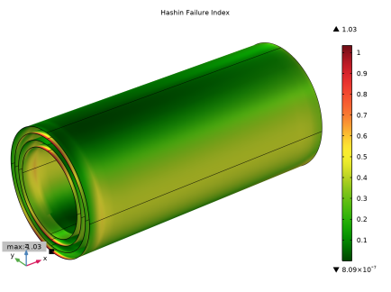
In the Settings window for Evaluation Group, type Hashin Failure Indexes (Study: Macromechanics (Global Response)) in the Label text field.
|
|
3
|
|
1
|
Right-click Hashin Failure Indexes (Study: Macromechanics (Global Response)) and choose Maximum > Volume Maximum.
|
|
2
|
In the Settings window for Volume Maximum, click Add Expression in the upper-right corner of the Expressions section. From the menu, choose Component: Macromechanics (Global Response) (comp2) > Layered Shell > Safety > Hashin > lshell.lemm1.sf1.f_ifT - Hashin fiber tensile failure index - 1.
|
|
3
|
Click Add Expression in the upper-right corner of the Expressions section. From the menu, choose Component: Macromechanics (Global Response) (comp2) > Layered Shell > Safety > Hashin > lshell.lemm1.sf1.f_ifC - Hashin fiber compressive failure index - 1.
|
|
4
|
Click Add Expression in the upper-right corner of the Expressions section. From the menu, choose Component: Macromechanics (Global Response) (comp2) > Layered Shell > Safety > Hashin > lshell.lemm1.sf1.f_imT - Hashin matrix tensile failure index - 1.
|
|
5
|
Click Add Expression in the upper-right corner of the Expressions section. From the menu, choose Component: Macromechanics (Global Response) (comp2) > Layered Shell > Safety > Hashin > lshell.lemm1.sf1.f_imC - Hashin matrix compressive failure index - 1.
|
|
6
|
Click Add Expression in the upper-right corner of the Expressions section. From the menu, choose Component: Macromechanics (Global Response) (comp2) > Layered Shell > Safety > Hashin > lshell.lemm1.sf1.f_iiT - Hashin interlaminar tensile failure index - 1.
|
|
7
|
Click Add Expression in the upper-right corner of the Expressions section. From the menu, choose Component: Macromechanics (Global Response) (comp2) > Layered Shell > Safety > Hashin > lshell.lemm1.sf1.f_iiC - Hashin interlaminar compressive failure index - 1.
|
|
1
|
In the Model Builder window, click Hashin Failure Indexes (Study: Macromechanics (Global Response)).
|
|
2
|
|
3
|
Select the Transpose checkbox.
|
|
4
|
|
1
|
|
2
|
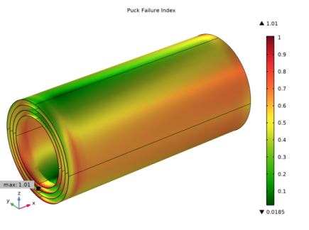
In the Settings window for Evaluation Group, type Puck Failure Indexes (Study: Macromechanics (Global Response)) in the Label text field.
|
|
3
|
|
1
|
Right-click Puck Failure Indexes (Study: Macromechanics (Global Response)) and choose Maximum > Volume Maximum.
|
|
2
|
In the Settings window for Volume Maximum, click Add Expression in the upper-right corner of the Expressions section. From the menu, choose Component: Macromechanics (Global Response) (comp2) > Layered Shell > Safety > Puck > lshell.lemm1.sf2.f_ifT - Puck fiber tensile failure index - 1.
|
|
3
|
Click Add Expression in the upper-right corner of the Expressions section. From the menu, choose Component: Macromechanics (Global Response) (comp2) > Layered Shell > Safety > Puck > lshell.lemm1.sf2.f_ifC - Puck fiber compressive failure index - 1.
|
|
4
|
Click Add Expression in the upper-right corner of the Expressions section. From the menu, choose Component: Macromechanics (Global Response) (comp2) > Layered Shell > Safety > Puck > lshell.lemm1.sf2.f_imA - Puck interfiber mode A failure index - 1.
|
|
5
|
Click Add Expression in the upper-right corner of the Expressions section. From the menu, choose Component: Macromechanics (Global Response) (comp2) > Layered Shell > Safety > Puck > lshell.lemm1.sf2.f_imB - Puck interfiber mode B failure index - 1.
|
|
6
|
Click Add Expression in the upper-right corner of the Expressions section. From the menu, choose Component: Macromechanics (Global Response) (comp2) > Layered Shell > Safety > Puck > lshell.lemm1.sf2.f_imC - Puck interfiber mode C failure index - 1.
|
|
1
|
|
2
|
|
3
|
Select the Transpose checkbox.
|
|
4
|
|
1
|
In the Model Builder window, under Results, Ctrl-click to select Stress (lshell), Stress, Slice (lshell), Stress, Through Thickness (lshell), Hashin Failure Index, and Puck Failure Index.
|
|
2
|
Right-click and choose Group.
|
|
1
|
|
2
|
|
3
|
Locate the Parameters section. In the table, enter the following settings:
|
|
4
|
|
5
|
|
6
|
|
8
|
|
9
|
|
11
|
|
12
|
|
14
|
|
15
|
|
17
|
|
18
|
|
1
|
|
2
|
|
3
|
In the Settings window for Component, type Component: Micromechanics (Local Response) in the Label text field.
|
|
1
|
|
2
|
Select the object pi1 only.
|
|
3
|
|
4
|
|
5
|
Click
|
|
1
|
|
2
|
|
3
|
|
1
|
|
2
|
|
3
|
Find the Coordinate names subsection. From the Create first tangent direction from list, choose Rotated System 4 (sys4).
|
|
4
|
|
1
|
|
2
|
|
3
|
Click
|
|
4
|
Browse to the model’s Application Libraries folder and double-click the file composite_multiscale_variables.txt.
|
|
1
|
In the Model Builder window, expand the Component: Micromechanics (Local Response) (comp3) > Solid Mechanics (solid2) node, then click Linear Elastic Material 1.
|
|
2
|
|
3
|
|
1
|
|
2
|
|
4
|
|
5
|
|
6
|
|
1
|
|
2
|
|
4
|
|
5
|
|
6
|
|
1
|
|
2
|
|
3
|
|
4
|
|
5
|
|
1
|
In the Model Builder window, under Component: Micromechanics (Local Response) (comp3) > Solid Mechanics (solid2) click Cell Periodicity 1.
|
|
2
|
|
3
|
|
4
|
|
5
|
|
6
|
|
7
|
|
8
|
|
9
|
|
1
|
In the Model Builder window, expand the Component: Micromechanics (Local Response) (comp3) > Mesh 1 node.
|
|
2
|
Right-click Component: Micromechanics (Local Response) (comp3) > Mesh 1 > Swept 1 and choose Build Selected.
|
|
1
|
|
2
|
Go to the Add Study window.
|
|
3
|
|
4
|
Find the Physics interfaces in study subsection. In the table, clear the Solve checkboxes for Solid Mechanics (solid) and Layered Shell (lshell).
|
|
5
|
Click the Add Study button in the window toolbar.
|
|
6
|
|
1
|
In the Settings window for Study, type Study: Micromechanics (Local Response) in the Label text field.
|
|
2
|
|
1
|
|
2
|
|
3
|
|
4
|
Click
|
|
1
|
|
2
|
|
3
|
Click
|
|
1
|
|
2
|
|
3
|
Find the Values of variables not solved for subsection. From the Settings list, choose User controlled.
|
|
4
|
|
5
|
|
6
|
|
1
|
|
2
|
|
1
|
In the Model Builder window, expand the Micromechanics (Local Response) node, then click Stress, Unit Cell 1.
|
|
2
|
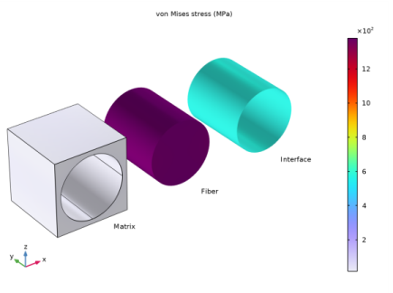
In the Settings window for 3D Plot Group, type Stress, Unit Cell (At First Material Point in Inner Layer) in the Label text field.
|
|
3
|
Locate the Data section. From the Dataset list, choose Study: Micromechanics (Local Response)/Parametric Solutions 1 (9) (sol3).
|
|
4
|
|
5
|
|
6
|
|
1
|
In the Model Builder window, expand the Stress, Unit Cell (At First Material Point in Inner Layer) node, then click Volume 1.
|
|
2
|
|
3
|
|
1
|
|
2
|
|
3
|
Click to select the
|
|
1
|
In the Model Builder window, under Results > Micromechanics (Local Response) > Stress, Unit Cell (At First Material Point in Inner Layer) click Volume 2.
|
|
2
|
|
3
|
|
1
|
|
2
|
|
3
|
Click to select the
|
|
1
|
In the Model Builder window, under Results > Micromechanics (Local Response) > Stress, Unit Cell (At First Material Point in Inner Layer) click Surface 1.
|
|
2
|
|
3
|
|
1
|
|
2
|
|
3
|
Click to select the
|
|
5
|
|
6
|
|
1
|
|
2
|
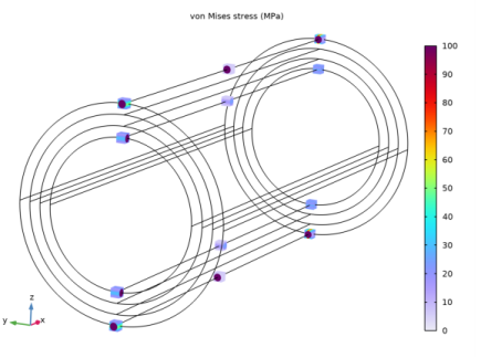
In the Settings window for 3D Plot Group, type Stress, Unit Cell (At Multiple Material Points) in the Label text field.
|
|
3
|
Locate the Data section. From the Dataset list, choose Study: Micromechanics (Local Response)/Parametric Solutions 1 (9) (sol3).
|
|
4
|
|
5
|
|
6
|
Clear the Parameter indicator text field.
|
|
7
|
|
1
|
|
2
|
|
3
|
From the Dataset list, choose Study: Micromechanics (Local Response)/Parametric Solutions 1 (9) (sol3).
|
|
4
|
|
5
|
|
6
|
|
7
|
|
8
|
|
9
|
|
10
|
|
11
|
|
12
|
|
13
|
|
14
|
|
1
|
|
2
|
|
3
|
|
4
|
|
5
|
|
1
|
In the Model Builder window, under Results > Micromechanics (Local Response) > Stress, Unit Cell (At Multiple Material Points) right-click Surface 1 and choose Duplicate.
|
|
2
|
|
3
|
|
4
|
|
1
|
|
2
|
|
3
|
|
1
|
|
2
|
|
3
|
|
1
|
|
2
|
|
3
|
|
1
|
In the Model Builder window, under Results > Micromechanics (Local Response) > Stress, Unit Cell (At Multiple Material Points) right-click Surface 4 and choose Duplicate.
|
|
2
|
|
3
|
|
1
|
|
2
|
|
3
|
|
1
|
|
2
|
|
3
|
|
4
|
|
1
|
|
2
|
|
3
|
|
1
|
|
2
|
|
3
|
|
1
|
|
2
|
|
3
|
|
1
|
|
2
|
|
3
|
|
1
|
In the Model Builder window, under Results > Micromechanics (Local Response) > Stress, Unit Cell (At Multiple Material Points) right-click Surface 10 and choose Duplicate.
|
|
2
|
|
3
|
|
1
|
|
2
|
|
3
|
|
1
|
In the Model Builder window, right-click Stress, Unit Cell (At Multiple Material Points) and choose Line.
|
|
2
|
|
3
|
|
4
|
|
5
|
|
6
|
|
1
|
|
2
|
|
3
|
|
4
|
|
5
|
|
1
|
In the Model Builder window, right-click Stress, Unit Cell (At First Material Point in Inner Layer) and choose Duplicate.
|
|
2
|
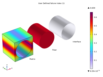
In the Settings window for 3D Plot Group, type User Defined Failure Indexes (At First Material Point in Inner Layer) in the Label text field.
|
|
3
|
|
4
|
|
1
|
In the Model Builder window, expand the User Defined Failure Indexes (At First Material Point in Inner Layer) node, then click Volume 1.
|
|
2
|
In the Settings window for Volume, click Replace Expression in the upper-right corner of the Expression section. From the menu, choose Component: Micromechanics (Local Response) (comp3) > Solid Mechanics > Safety > User defined > solid2.lemm1.sf2.f_i - User-defined failure index - 1.
|
|
1
|
|
2
|
In the Settings window for Volume, click Replace Expression in the upper-right corner of the Expression section. From the menu, choose Component: Micromechanics (Local Response) (comp3) > Solid Mechanics > Safety > User defined > solid2.lemm1.sf1.f_i - User-defined failure index - 1.
|
|
1
|
|
2
|
In the Settings window for Surface, click Replace Expression in the upper-right corner of the Expression section. From the menu, choose Component: Micromechanics (Local Response) (comp3) > Solid Mechanics > Safety > User defined > solid2.tl1.lemm1.sf1.f_i - User-defined failure index - 1.
|
|
1
|
|
2
|
In the Model Builder window, click User Defined Failure Indexes (At First Material Point in Inner Layer).
|
|
3
|
|
1
|
Right-click User Defined Failure Indexes (At First Material Point in Inner Layer) and choose Duplicate.
|
|
2
|
In the Settings window for 3D Plot Group, type User Defined Failure Indexes (At First Material Point in Outer Layer) in the Label text field.
|
|
3
|
|
4
|
|
5
|
|
1
|
|
2
|
In the Settings window for Evaluation Group, type User Defined Failure Indexes at First Material Point in Inner Layer (Study: Micromechanics (Local Response)) in the Label text field.
|
|
3
|
Locate the Data section. From the Dataset list, choose Study: Micromechanics (Local Response)/Parametric Solutions 1 (9) (sol3).
|
|
4
|
|
5
|
|
1
|
Right-click User Defined Failure Indexes at First Material Point in Inner Layer (Study: Micromechanics (Local Response)) and choose Maximum > Volume Maximum.
|
|
3
|
In the Settings window for Volume Maximum, click Replace Expression in the upper-right corner of the Expressions section. From the menu, choose Component: Micromechanics (Local Response) (comp3) > Solid Mechanics > Safety > User defined > solid2.lemm1.sf2.f_i - User-defined failure index - 1.
|
|
4
|
Locate the Expressions section. In the table, enter the following settings:
|
|
1
|
In the Model Builder window, right-click User Defined Failure Indexes at First Material Point in Inner Layer (Study: Micromechanics (Local Response)) and choose Maximum > Volume Maximum.
|
|
3
|
In the Settings window for Volume Maximum, click Replace Expression in the upper-right corner of the Expressions section. From the menu, choose Component: Micromechanics (Local Response) (comp3) > Solid Mechanics > Safety > User defined > solid2.lemm1.sf1.f_i - User-defined failure index - 1.
|
|
4
|
Locate the Expressions section. In the table, enter the following settings:
|
|
1
|
Right-click User Defined Failure Indexes at First Material Point in Inner Layer (Study: Micromechanics (Local Response)) and choose Maximum > Surface Maximum.
|
|
2
|
|
3
|
|
4
|
Click Replace Expression in the upper-right corner of the Expressions section. From the menu, choose Component: Micromechanics (Local Response) (comp3) > Solid Mechanics > Safety > User defined > solid2.tl1.lemm1.sf1.f_i - User-defined failure index - 1.
|
|
5
|
Locate the Expressions section. In the table, enter the following settings:
|
|
1
|
In the Model Builder window, click User Defined Failure Indexes at First Material Point in Inner Layer (Study: Micromechanics (Local Response)).
|
|
2
|
|
3
|
Select the Transpose checkbox.
|
|
4
|
|
5
|
In the User Defined Failure Indexes at First Material Point in Inner Layer (Study: Micromechanics (Local Response)) toolbar, click
|
|
1
|
Right-click User Defined Failure Indexes at First Material Point in Inner Layer (Study: Micromechanics (Local Response)) and choose Duplicate.
|
|
2
|
In the Settings window for Evaluation Group, type User Defined Failure Indexes at First Material Point in Outer Layer (Study: Micromechanics (Local Response)) in the Label text field.
|
|
3
|
|
4
|
In the User Defined Failure Indexes at First Material Point in Outer Layer (Study: Micromechanics (Local Response)) toolbar, click
|