|
|
|
|
|
|
•
|
Modeling a composite laminate as a layered shell requires a surface geometry, in general referred to as a base surface, and a Layered Material node which adds an extra dimension (1D) to the base surface geometry in the surface normal direction. You can use the Layered Material functionality to model several layers stacked on top of each other having different thicknesses, material properties, and fiber orientations. You can optionally specify the interface materials between the layers, and control the number of through-thickness mesh elements for each layer.
|
|
•
|
The third direction for the selected coordinate system in the Single Layer Material, Layered Material Link, or Layered Material Stack represents the normal direction of the Layered Shell or Shell physics. This is also the direction in which the layer stacking is interpreted from bottom to top, and therefore, it is crucial to know it during modeling. There are two ways to achieve this:
|
|
-
|
Using physics symbols: Go to the physics settings, find the Physics Symbols section, and select the Enable physics symbols checkbox. Then go to the material feature, for instance, Linear Elastic Material, to see the normal direction represented by green arrows in the geometry.
|
|
-
|
Using result templates: When a solution dataset is available, use the result template Thickness and Orientation to plot the normal direction.
|
|
•
|
To run the analysis for different layered materials and compare the results, all the layered materials can be defined using a Switch node in Global Materials. This Switch node can be selected in the Layered Material Link node and a Material Sweep node is added in the study.
|
|
•
|
From a constitutive model point of view, you can either use the Layerwise (LW) theory based Layered Shell interface, or the Equivalent Single Layer (ESL) theory based Linear Elastic Material, Layered node in the Shell interface. The laminated composite presented in the current model is modeled using a Layered Shell interface.
|
|
1
|
|
2
|
|
3
|
Right-click and choose Add Physics.
|
|
4
|
|
5
|
Right-click and choose Add Physics.
|
|
6
|
In the Select Physics tree, select Acoustics > Pressure Acoustics > Pressure Acoustics, Frequency Domain (acpr).
|
|
7
|
Right-click and choose Add Physics.
|
|
8
|
|
9
|
Right-click and choose Add Physics.
|
|
10
|
Click
|
|
11
|
|
12
|
Click
|
|
1
|
|
2
|
|
3
|
|
4
|
Browse to the model’s Application Libraries folder and double-click the file composite_dome_tweeter_freq_geom_parameters.txt.
|
|
1
|
|
2
|
|
3
|
|
4
|
Browse to the model’s Application Libraries folder and double-click the file composite_dome_tweeter_freq_model_parameters.txt.
|
|
1
|
|
2
|
In the Settings window for Interpolation, type Interpolation Function: Lp Data in the Label text field.
|
|
3
|
|
4
|
Click
|
|
5
|
Browse to the model’s Application Libraries folder and double-click the file composite_dome_tweeter_freq_Lp_data.txt.
|
|
6
|
Locate the Data Column Settings section. In the table, click to select the cell at row number 1 and column number 1.
|
|
7
|
|
9
|
|
10
|
|
12
|
|
13
|
|
15
|
|
16
|
|
17
|
Locate the Interpolation and Extrapolation section. From the Interpolation list, choose Cubic spline.
|
|
18
|
|
1
|
|
2
|
In the Settings window for Interpolation, type Interpolation Function: Z Data in the Label text field.
|
|
3
|
|
4
|
Click
|
|
5
|
Browse to the model’s Application Libraries folder and double-click the file composite_dome_tweeter_freq_Z_data.txt.
|
|
6
|
Locate the Data Column Settings section. In the table, click to select the cell at row number 1 and column number 1.
|
|
7
|
|
9
|
|
10
|
|
12
|
|
13
|
|
15
|
|
16
|
|
17
|
|
1
|
|
2
|
Go to the Add Material window.
|
|
3
|
|
4
|
Right-click and choose Add to Global Materials.
|
|
5
|
|
6
|
Right-click and choose Add to Global Materials.
|
|
7
|
|
8
|
Right-click and choose Add to Global Materials.
|
|
9
|
|
10
|
Right-click and choose Add to Global Materials.
|
|
11
|
|
1
|
In the Model Builder window, under Global Definitions right-click Materials and choose Blank Material.
|
|
2
|
|
3
|
Click to expand the Material Properties section. In the Material properties tree, select Basic Properties > Density.
|
|
4
|
Right-click and choose Add to Material.
|
|
5
|
|
6
|
Right-click and choose Add to Material.
|
|
7
|
|
8
|
Right-click and choose Add to Material.
|
|
9
|
Locate the Material Contents section. In the table, enter the following settings:
|
|
1
|
|
2
|
|
3
|
Click to expand the Material Properties section. In the Material properties tree, select Basic Properties > Porosity.
|
|
4
|
Right-click and choose Add to Material.
|
|
5
|
|
6
|
Right-click and choose Add This Property Group to Material.
|
|
7
|
Locate the Material Contents section. In the table, enter the following settings:
|
|
8
|
|
9
|
|
10
|
|
11
|
In the Application Libraries window, select Composite Materials Module > Dynamics and Vibration > composite_dome_tweeter_eigen in the tree.
|
|
12
|
Click
|
|
13
|
|
14
|
Click OK.
|
|
1
|
|
2
|
|
3
|
Locate the Layer Definition section. In the table, enter the following settings:
|
|
1
|
|
2
|
In the Settings window for Layered Material, type Layered Material: Glass Fiber in the Label text field.
|
|
3
|
Locate the Layer Definition section. In the table, enter the following settings:
|
|
1
|
|
2
|
In the Settings window for Layered Material, type Layered Material: Titanium in the Label text field.
|
|
3
|
Locate the Layer Definition section. In the table, enter the following settings:
|
|
1
|
|
2
|
In the Settings window for Layered Material, type Layered Material: Composite Material 1 in the Label text field.
|
|
3
|
Locate the Layer Definition section. In the table, enter the following settings:
|
|
1
|
|
2
|
In the Settings window for Layered Material, type Layered Material: Composite Material 2 in the Label text field.
|
|
3
|
Locate the Layer Definition section. In the table, enter the following settings:
|
|
1
|
|
2
|
|
3
|
|
1
|
|
2
|
|
3
|
Click
|
|
4
|
Browse to the model’s Application Libraries folder and double-click the file composite_dome_tweeter_freq_geom_sequence.mphbin.
|
|
5
|
Click
|
|
6
|
|
1
|
|
2
|
|
3
|
|
4
|
|
5
|
Click OK.
|
|
1
|
|
2
|
|
3
|
|
4
|
|
5
|
Click OK.
|
|
1
|
|
2
|
|
3
|
|
4
|
|
5
|
Click OK.
|
|
1
|
|
2
|
|
3
|
|
4
|
Click
|
|
5
|
|
6
|
Click OK.
|
|
1
|
|
2
|
|
3
|
|
4
|
Click
|
|
5
|
|
6
|
Click OK.
|
|
1
|
|
2
|
|
3
|
|
4
|
Click
|
|
5
|
|
6
|
Click OK.
|
|
1
|
|
2
|
|
3
|
|
4
|
|
5
|
In the Add dialog, in the Selections to add list, choose Rubber Boundaries, Glass Fiber Boundaries, and Diaphragm Boundaries.
|
|
6
|
Click OK.
|
|
7
|
|
1
|
|
2
|
|
3
|
|
4
|
Click
|
|
5
|
|
6
|
Click OK.
|
|
1
|
|
2
|
|
3
|
|
4
|
Click
|
|
5
|
|
6
|
Click OK.
|
|
1
|
|
2
|
In the Settings window for Explicit, type Acoustic-Layered Shell Boundaries in the Label text field.
|
|
3
|
|
4
|
Click
|
|
5
|
|
6
|
Click OK.
|
|
1
|
|
2
|
|
3
|
|
4
|
Click
|
|
5
|
|
6
|
Click OK.
|
|
1
|
|
2
|
|
3
|
|
4
|
Click
|
|
5
|
In the Paste Selection dialog, type 1 2 4 5 7 8 10 11 14 17 20 23 34 44 53 66 67 68 69 70 71 72 in the Selection text field.
|
|
6
|
Click OK.
|
|
1
|
|
2
|
|
3
|
|
4
|
Click
|
|
5
|
In the Paste Selection dialog, type 12, 13, 44, 47, 50, 55, 116, 118, 120, 122 in the Selection text field.
|
|
6
|
Click OK.
|
|
1
|
|
2
|
|
3
|
|
1
|
|
2
|
|
1
|
In the Model Builder window, under Component 1 (comp1) right-click Materials and choose More Materials > Material Link.
|
|
2
|
|
3
|
|
1
|
|
2
|
|
3
|
|
4
|
|
1
|
|
2
|
In the Settings window for Layered Material Link, type Layered Material Link: Rubber in the Label text field.
|
|
3
|
|
4
|
|
1
|
|
2
|
In the Settings window for Layered Material Link, type Layered Material Link: Glass Fiber in the Label text field.
|
|
3
|
|
4
|
Locate the Layered Material Settings section. From the Material list, choose Layered Material: Glass Fiber (lmat2).
|
|
1
|
|
2
|
In the Settings window for Layered Material Link, type Layered Material Link: Diaphragm in the Label text field.
|
|
3
|
|
4
|
Locate the Layered Material Settings section. From the Material list, choose Material Switch 1 (sw1).
|
|
5
|
|
1
|
In the Model Builder window, under Component 1 (comp1) > Definitions click Boundary System 1 (sys1).
|
|
2
|
|
3
|
|
1
|
|
2
|
|
3
|
|
1
|
In the Model Builder window, under Component 1 (comp1) > Layered Shell (lshell) click Linear Elastic Material 1.
|
|
2
|
|
3
|
|
1
|
|
2
|
|
3
|
|
4
|
|
1
|
|
2
|
|
3
|
|
4
|
|
5
|
In the Selection table, enter the following settings:
|
|
1
|
|
2
|
|
3
|
|
4
|
In the Selection table, enter the following settings:
|
|
1
|
|
2
|
|
3
|
|
1
|
|
2
|
|
3
|
|
1
|
|
2
|
|
3
|
|
1
|
|
2
|
|
3
|
|
4
|
|
5
|
|
1
|
|
2
|
|
3
|
|
1
|
In the Model Builder window, under Component 1 (comp1) click Pressure Acoustics, Frequency Domain (acpr).
|
|
2
|
In the Settings window for Pressure Acoustics, Frequency Domain, locate the Domain Selection section.
|
|
3
|
|
1
|
|
2
|
|
3
|
|
4
|
Locate the Poroacoustics Model section. From the Poroacoustics model list, choose Johnson–Champoux–Allard (JCA).
|
|
5
|
Locate the Porous Matrix Properties section. From the Porous elastic material list, choose Foam (mat6).
|
|
1
|
|
2
|
|
3
|
|
1
|
|
2
|
|
3
|
|
4
|
Locate the Exterior Field Calculation section. From the Symmetry type list, choose Sector symmetry with one symmetry plane.
|
|
5
|
|
6
|
|
1
|
|
2
|
|
3
|
|
1
|
|
2
|
|
4
|
|
1
|
|
2
|
|
4
|
|
1
|
|
2
|
|
4
|
|
1
|
|
2
|
|
4
|
|
1
|
|
2
|
|
4
|
|
1
|
|
2
|
In the Settings window for Acoustic–Structure Boundary, type Acoustic-Solid Boundary in the Label text field.
|
|
3
|
|
4
|
|
1
|
|
2
|
In the Settings window for Acoustic–Structure Boundary, type Acoustic-Layered Shell Boundary in the Label text field.
|
|
3
|
Locate the Boundary Selection section. From the Selection list, choose Acoustic–Layered Shell Boundaries.
|
|
1
|
|
2
|
|
3
|
|
1
|
|
2
|
|
3
|
Click the Custom button.
|
|
4
|
Locate the Geometric Entity Selection section. From the Selection list, choose Diaphragm Boundaries.
|
|
5
|
Locate the Element Size Parameters section.
|
|
6
|
|
7
|
|
1
|
|
2
|
|
3
|
|
1
|
|
2
|
|
3
|
|
4
|
|
1
|
|
2
|
|
3
|
|
4
|
|
1
|
|
2
|
|
3
|
|
1
|
|
2
|
|
3
|
|
4
|
|
1
|
|
2
|
|
3
|
Click the Custom button.
|
|
4
|
|
5
|
|
6
|
|
7
|
Click
|
|
1
|
|
2
|
|
3
|
|
1
|
|
2
|
|
3
|
Click
|
|
1
|
|
2
|
|
3
|
Click
|
|
4
|
|
5
|
|
6
|
|
7
|
|
8
|
Click Replace.
|
|
9
|
|
10
|
|
11
|
|
1
|
|
2
|
|
3
|
In the Model Builder window, expand the Study: Frequency Response > Solver Configurations > Solution 1 (sol1) > Stationary Solver 1 node.
|
|
4
|
Right-click Study: Frequency Response > Solver Configurations > Solution 1 (sol1) > Stationary Solver 1 > Suggested Iterative Solver (GMRES with GMG and Direct Precond.) (asb1_asb2) and choose Enable.
|
|
5
|
|
6
|
|
7
|
|
8
|
In the Model Builder window, expand the Study: Frequency Response > Solver Configurations > Solution 1 (sol1) > Stationary Solver 1 > Suggested Iterative Solver (GMRES with GMG and Direct Precond.) (asb1_asb2) node, then click Direct Preconditioner 1.
|
|
9
|
|
10
|
|
11
|
|
12
|
In the Add dialog, in the Preconditioner variables list, choose Voltages (comp1.voltages), Currents (comp1.currents), and Currents, Time Derivatives (comp1.current_time).
|
|
13
|
Click OK.
|
|
14
|
|
1
|
|
2
|
|
3
|
Select the Only plot when requested checkbox.
|
|
1
|
|
2
|
Go to the Result Templates window.
|
|
3
|
In the tree, select Study: Frequency Response/Parametric Solutions 1 (sol2) > Layered Shell > Displacement (lshell).
|
|
4
|
Click the Add Result Template button in the window toolbar.
|
|
5
|
|
1
|
|
2
|
|
3
|
|
4
|
|
5
|
|
6
|
|
1
|
|
2
|
In the Settings window for 3D Plot Group, type Diaphragm Displacement (lshell) in the Label text field.
|
|
3
|
|
4
|
|
5
|
|
6
|
|
7
|
|
8
|
|
9
|
|
1
|
|
2
|
|
3
|
|
4
|
|
5
|
|
6
|
|
7
|
|
1
|
|
2
|
|
3
|
|
1
|
|
2
|
|
3
|
|
5
|
|
1
|
|
2
|
|
3
|
|
4
|
|
1
|
|
2
|
|
3
|
|
1
|
|
2
|
|
3
|
|
4
|
|
1
|
|
2
|
|
3
|
|
4
|
|
5
|
|
6
|
|
7
|
|
8
|
|
9
|
|
10
|
|
1
|
|
2
|
|
3
|
|
4
|
|
5
|
|
6
|
|
1
|
|
2
|
|
3
|
|
4
|
|
5
|
|
6
|
|
1
|
|
2
|
|
3
|
|
1
|
|
2
|
|
3
|
|
4
|
|
5
|
|
6
|
|
1
|
|
2
|
|
3
|
|
4
|
|
5
|
|
6
|
|
7
|
|
1
|
|
2
|
|
3
|
Click
|
|
4
|
|
5
|
Click OK.
|
|
1
|
|
2
|
|
3
|
|
1
|
|
2
|
|
3
|
|
1
|
|
2
|
|
3
|
|
5
|
|
1
|
|
2
|
|
3
|
|
4
|
|
1
|
|
2
|
|
3
|
|
1
|
|
2
|
|
3
|
|
4
|
|
5
|
|
1
|
|
2
|
|
3
|
|
1
|
|
2
|
|
3
|
|
1
|
|
2
|
|
1
|
In the Model Builder window, under Global Definitions click Interpolation Function: Lp Data (Lp1, Lp2, Lp3).
|
|
2
|
|
1
|
|
2
|
|
3
|
|
1
|
In the Model Builder window, under Global Definitions click Interpolation Function: Z Data (Zabs1, Zabs2, Zabs3).
|
|
2
|
|
1
|
|
2
|
|
3
|
|
1
|
|
2
|
|
3
|
|
4
|
Locate the Plot Settings section.
|
|
5
|
|
6
|
|
7
|
Click to expand the Number Format section. Locate the Legend section. From the Position list, choose Lower left.
|
|
1
|
|
2
|
|
3
|
|
4
|
|
5
|
|
6
|
Click to expand the Coloring and Style section. Find the Line style subsection. From the Line list, choose None.
|
|
7
|
|
8
|
|
9
|
|
10
|
|
1
|
|
2
|
|
1
|
|
2
|
|
1
|
|
2
|
|
1
|
|
2
|
|
1
|
|
2
|
|
3
|
|
4
|
Locate the Plot Settings section.
|
|
5
|
|
6
|
|
1
|
|
2
|
|
3
|
|
4
|
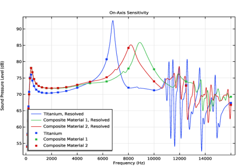
Locate the y-Axis Data section. In the table, enter the following settings:
|
|
5
|
|
6
|
Click to expand the Coloring and Style section. Find the Line style subsection. From the Line list, choose None.
|
|
7
|
|
8
|
|
9
|
|
1
|
|
2
|
|
1
|
|
2
|
|
1
|
|
2
|
|
1
|
|
2
|
|
1
|
|
2
|
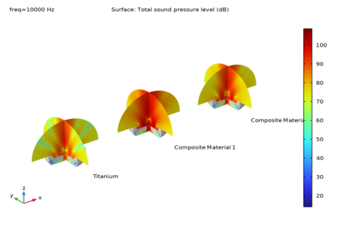
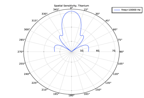
In the Settings window for Polar Plot Group, type Spatial Sensitivity, Titanium in the Label text field.
|
|
3
|
Locate the Data section. From the Dataset list, choose Study: Frequency Response/Parametric Solutions 1 (sol2).
|
|
4
|
|
5
|
|
6
|
|
7
|
|
8
|
|
9
|
|
10
|
|
1
|
|
2
|
|
3
|
|
4
|
|
5
|
|
6
|
|
7
|
|
8
|
|
9
|
|
10
|
|
11
|
|
12
|
|
13
|
|
1
|
|
2
|
|
1
|
|
2
|
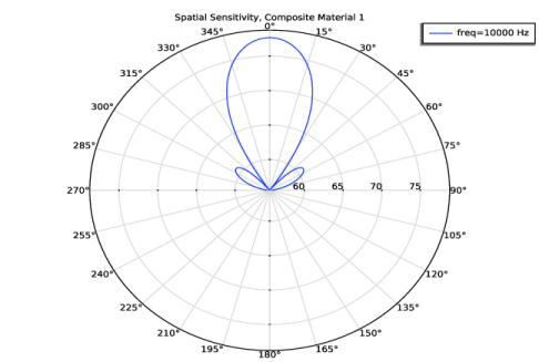
In the Settings window for Polar Plot Group, type Spatial Sensitivity, Composite Material 1 in the Label text field.
|
|
3
|
Locate the Data section. In the Values (Material Switch 1) list box, select Layered Material: Composite Material 1.
|
|
4
|
|
1
|
|
2
|
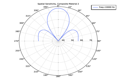
In the Settings window for Polar Plot Group, type Spatial Sensitivity, Composite Material 2 in the Label text field.
|
|
3
|
Locate the Data section. In the Values (Material Switch 1) list box, select Layered Material: Composite Material 2.
|
|
4
|
|
1
|
|
2
|
|
3
|
Locate the Data section. From the Dataset list, choose Study: Frequency Response/Parametric Solutions 1 (sol2).
|
|
4
|
|
5
|
|
6
|
|
7
|
|
8
|
|
1
|
|
2
|
|
3
|
|
4
|
|
5
|
|
6
|
|
7
|
|
8
|
|
9
|
|
10
|
|
11
|
|
1
|
|
2
|