|
|
|
|
|
|
{235,15} GPa
|
|
|
G12
|
27 GPa
|
|
•
|
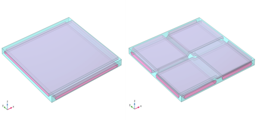
Modeling a composite laminate as a layered shell requires a surface geometry, in general referred to as a base surface, and a Layered Material node which adds an extra dimension (1D) to the base surface geometry in the surface normal direction. You can use the Layered Material functionality to model several layers stacked on top of each other having different thicknesses, material properties, and fiber orientations. You can optionally specify the interface materials between the layers, and control the number of through-thickness mesh elements for each layer.
|
|
•
|
The third direction for the selected coordinate system in the Single Layer Material, Layered Material Link, or Layered Material Stack represents the normal direction of the Layered Shell or Shell physics. This is also the direction in which the layer stacking is interpreted from bottom to top, and therefore, it is crucial to know it during modeling. There are two ways to achieve this:
|
|
-
|
Using physics symbols: Go to the physics settings, find the Physics Symbols section, and select the Enable physics symbols checkbox. Then go to the material feature, for instance, Linear Elastic Material, to see the normal direction represented by green arrows in the geometry.
|
|
-
|
Using result templates: When a solution dataset is available, use the result template Thickness and Orientation to plot the normal direction.
|
|
•
|
In order to run the analysis for various layered materials and compare the results, all the layered materials can be defined using a Switch node in Global Materials. This Switch node can be selected in the Layered Material Link node and a Material Sweep node is added in the study.
|
|
•
|
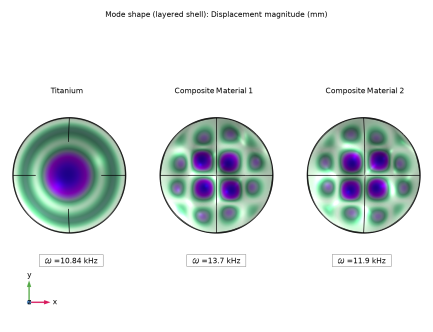
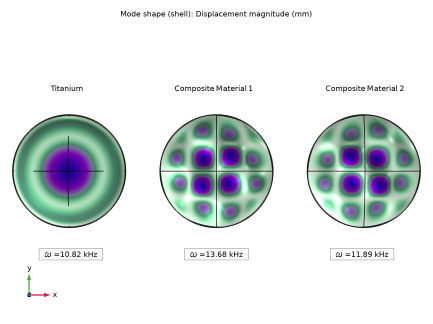
You can either use the Layerwise (LW) theory-based Layered Shell interface or the Equivalent Single Layer (ESL) theory-based Linear Elastic Material, Layered node in Shell interface.
|
|
•
|
The built-in Composites material library contains data for fiber and matrix constituents as well as for unidirectional and bidirectional laminae.
|
|
1
|
|
2
|
|
3
|
Click Add.
|
|
4
|
|
5
|
Click Add.
|
|
6
|
Click
|
|
1
|
|
2
|
|
1
|
In the Model Builder window, right-click Global Definitions and choose Geometry Parts > Part Libraries.
|
|
1
|
In the Part Libraries window, select COMSOL Multiphysics > Unit Cells and RVEs > Fiber Composites > bidirectional_non_crimp_fiber in the tree.
|
|
2
|
Click
|
|
1
|
In the Part Libraries window, select COMSOL Multiphysics > Unit Cells and RVEs > Fiber Composites > bidirectional_spread_tow_fiber in the tree.
|
|
2
|
Click
|
|
1
|
|
2
|
In the Settings window for Part Instance, type RUC 1: Bidirectional Non-Crimp Fiber Composite in the Label text field.
|
|
3
|
Locate the Input Parameters section. In the table, enter the following settings:
|
|
4
|
Click
|
|
1
|
|
2
|
In the Settings window for Part Instance, type RUC 2: Bidirectional Spread-Tow Fiber Composite in the Label text field.
|
|
3
|
Locate the Input Parameters section. In the table, enter the following settings:
|
|
4
|
Locate the Position and Orientation of Output section. Find the Displacement subsection. In the ywi text field, type 2[mm].
|
|
5
|
Click
|
|
6
|
|
7
|
|
8
|
Clear the Automatic detection of small details checkbox.
|
|
1
|
Go to the Add Material window.
|
|
2
|
|
3
|
Right-click and choose Add to Component 1 (comp1).
|
|
1
|
|
2
|
|
3
|
|
1
|
|
2
|
|
3
|
|
1
|
Go to the Add Material window.
|
|
2
|
|
3
|
Right-click and choose Add to Component 1 (comp1).
|
|
1
|
|
2
|
|
3
|
|
1
|
|
2
|
|
3
|
|
4
|
|
1
|
In the Model Builder window, under Component 1 (comp1) > Materials, Ctrl-click to select AS-4 carbon fiber 1 (mat2) and Epoxy polymer 1 (mat4).
|
|
2
|
Right-click and choose Group.
|
|
1
|
|
2
|
|
4
|
|
1
|
|
2
|
|
3
|
Locate the Domain Selection section. From the Selection list, choose All (RUC 1: Bidirectional Non-Crimp Fiber Composite).
|
|
1
|
In the Model Builder window, under Component 1 (comp1) > Solid Mechanics: RUC 1 (solid) click Linear Elastic Material 1.
|
|
2
|
|
3
|
|
1
|
Right-click Component 1 (comp1) > Solid Mechanics: RUC 1 (solid) > Linear Elastic Material 1 and choose Duplicate.
|
|
2
|
|
3
|
Click
|
|
5
|
Locate the Coordinate System Selection section. From the Coordinate system list, choose Base Vector System 2 (sys2).
|
|
1
|
|
2
|
|
3
|
|
4
|
|
5
|
Select the Compute elasticity matrix, standard notation checkbox.
|
|
6
|
|
7
|
|
8
|
|
9
|
|
10
|
Click OK.
|
|
11
|
|
12
|
|
1
|
|
2
|
|
3
|
|
4
|
|
5
|
Locate the Destination Selection section. From the Selection list, choose Pair 1, Destination (RUC 1: Bidirectional Non-Crimp Fiber Composite).
|
|
6
|
|
1
|
|
2
|
|
3
|
|
4
|
|
5
|
Locate the Destination Selection section. From the Selection list, choose Pair 2, Destination (RUC 1: Bidirectional Non-Crimp Fiber Composite).
|
|
6
|
|
1
|
|
2
|
|
3
|
|
4
|
|
5
|
Locate the Destination Selection section. From the Selection list, choose Pair 3, Destination (RUC 1: Bidirectional Non-Crimp Fiber Composite).
|
|
6
|
|
1
|
|
2
|
In the Settings window for Cell Periodicity, click Automated Model Setup in the upper-right corner of the Periodicity Settings section. From the menu, choose Create Load Groups and Study to generate load groups and a study node.
|
|
1
|
|
2
|
|
3
|
Locate the Domain Selection section. From the Selection list, choose All (RUC 2: Bidirectional Spread-Tow Fiber Composite).
|
|
1
|
In the Model Builder window, under Component 1 (comp1) > Solid Mechanics: RUC 2 (solid2) click Linear Elastic Material 1.
|
|
2
|
|
3
|
|
1
|
Right-click Component 1 (comp1) > Solid Mechanics: RUC 2 (solid2) > Linear Elastic Material 1 and choose Duplicate.
|
|
2
|
|
3
|
Click
|
|
5
|
Locate the Coordinate System Selection section. From the Coordinate system list, choose Base Vector System 2 (sys2).
|
|
1
|
|
2
|
|
3
|
|
4
|
|
5
|
Select the Compute elasticity matrix, standard notation checkbox.
|
|
6
|
|
7
|
|
1
|
|
2
|
|
3
|
|
4
|
|
5
|
Locate the Destination Selection section. From the Selection list, choose Pair 1, Destination (RUC 2: Bidirectional Spread-Tow Fiber Composite).
|
|
6
|
|
1
|
|
2
|
|
3
|
|
4
|
|
5
|
Locate the Destination Selection section. From the Selection list, choose Pair 2, Destination (RUC 2: Bidirectional Spread-Tow Fiber Composite).
|
|
6
|
|
1
|
|
2
|
|
3
|
|
4
|
|
5
|
Locate the Destination Selection section. From the Selection list, choose Pair 3, Destination (RUC 2: Bidirectional Spread-Tow Fiber Composite).
|
|
6
|
|
1
|
|
2
|
In the Settings window for Cell Periodicity, click Automated Model Setup in the upper-right corner of the Periodicity Settings section. From the menu, choose Create Load Groups and Study to generate load groups and a study node.
|
|
1
|
|
2
|
|
3
|
Click the Custom button.
|
|
4
|
|
5
|
|
6
|
|
7
|
Click
|
|
1
|
|
2
|
|
1
|
In the Model Builder window, expand the Cell Periodicity Study: RUC 1 node, then click Step 1: Stationary.
|
|
2
|
|
3
|
Select the Modify model configuration for study step checkbox.
|
|
4
|
|
5
|
Right-click and choose Disable in Model.
|
|
1
|
|
2
|
|
1
|
|
2
|
|
3
|
Select the Modify model configuration for study step checkbox.
|
|
4
|
|
5
|
Right-click and choose Disable in Model.
|
|
1
|
|
2
|
|
3
|
|
4
|
|
5
|
Select the Apply to dataset edges checkbox.
|
|
6
|
|
7
|
|
8
|
|
1
|
|
2
|
|
3
|
|
4
|
|
5
|
Select the Apply to dataset edges checkbox.
|
|
6
|
|
7
|
|
8
|
|
1
|
In the Model Builder window, under Component 1 (comp1) > Solid Mechanics: RUC 1 (solid) click Cell Periodicity 1.
|
|
2
|
In the Settings window for Cell Periodicity, click Automated Model Setup in the upper-right corner of the Periodicity Settings section. From the menu, choose Create Material by Value to generate a global material node with computed density and elastic properties.
|
|
1
|
In the Model Builder window, expand the Global Definitions > Materials node, then click Homogeneous Material (solidcp1mat).
|
|
2
|
|
1
|
In the Model Builder window, under Component 1 (comp1) > Solid Mechanics: RUC 2 (solid2) click Cell Periodicity 1.
|
|
2
|
In the Settings window for Cell Periodicity, click Automated Model Setup in the upper-right corner of the Periodicity Settings section. From the menu, choose Create Material by Value to generate a global material node with computed density and elastic properties.
|
|
1
|
In the Model Builder window, under Global Definitions > Materials click Homogeneous Material (solid2cp1mat).
|
|
2
|
|
1
|
|
2
|
|
1
|
|
2
|
|
3
|
|
1
|
|
2
|
|
3
|
|
4
|
|
5
|
|
6
|
|
7
|
Select the Clockwise checkbox.
|
|
1
|
|
2
|
|
3
|
|
4
|
|
5
|
|
6
|
|
7
|
|
8
|
|
1
|
|
2
|
|
3
|
|
1
|
Go to the Add Material window.
|
|
2
|
|
3
|
Right-click and choose Add to Global Materials.
|
|
4
|
|
1
|
|
2
|
|
1
|
|
2
|
|
1
|
|
2
|
|
1
|
In the Model Builder window, under Component 2 (comp2) right-click Materials and choose Layers > Layered Material Link.
|
|
2
|
|
3
|
|
1
|
In the Model Builder window, under Component 2 (comp2) > Definitions click Boundary System 3 (sys3).
|
|
2
|
|
3
|
|
1
|
|
2
|
Go to the Add Physics window.
|
|
3
|
|
4
|
Click the Add to Component 2 button in the window toolbar.
|
|
5
|
|
6
|
Click the Add to Component 2 button in the window toolbar.
|
|
7
|
|
1
|
|
2
|
|
3
|
|
4
|
|
1
|
|
1
|
In the Model Builder window, under Component 2 (comp2) > Layered Shell (lshell) click Linear Elastic Material 1.
|
|
2
|
|
3
|
|
1
|
|
1
|
|
2
|
|
3
|
|
4
|
|
1
|
|
3
|
|
1
|
|
3
|
|
4
|
Click to select the
|
|
6
|
Click
|
|
1
|
|
2
|
|
3
|
Click to select the
|
|
5
|
|
6
|
Click
|
|
8
|
Click
|
|
1
|
|
2
|
Go to the Add Study window.
|
|
3
|
|
4
|
Click the Add Study button in the window toolbar.
|
|
5
|
|
6
|
Click the Add Study button in the window toolbar.
|
|
7
|
|
1
|
|
2
|
|
3
|
Click
|
|
1
|
|
2
|
|
3
|
|
4
|
In the Solve for column of the table, under Component 2 (comp2), clear the checkbox for Layered Shell (lshell).
|
|
1
|
|
2
|
|
1
|
|
2
|
|
3
|
Click
|
|
1
|
|
2
|
|
3
|
|
4
|
In the Solve for column of the table, under Component 2 (comp2), clear the checkbox for Shell (shell).
|
|
1
|
|
2
|
|
3
|
|
4
|
|
5
|
|
6
|
Clear the Parameter indicator text field.
|
|
7
|
|
8
|
|
1
|
|
2
|
|
3
|
|
4
|
|
5
|
|
1
|
|
2
|
|
3
|
|
4
|
|
5
|
|
1
|
|
2
|
|
3
|
|
4
|
Select the LaTeX markup checkbox.
|
|
5
|
|
6
|
|
7
|
|
8
|
|
9
|
Select the Show frame checkbox.
|
|
10
|
|
1
|
|
2
|
|
3
|
|
4
|
|
5
|
|
1
|
|
2
|
|
3
|
|
4
|
|
1
|
|
2
|
|
3
|
|
5
|
|
6
|
|
1
|
|
2
|
|
3
|
|
1
|
|
2
|
|
3
|
|
4
|
|
5
|
|
6
|
Clear the Parameter indicator text field.
|
|
7
|
|
8
|
|
1
|
|
2
|
|
3
|
|
4
|
|
5
|
|
1
|
|
2
|
|
3
|
|
1
|
|
2
|
|
3
|
|
4
|
Select the LaTeX markup checkbox.
|
|
5
|
|
6
|
|
7
|
|
8
|
|
9
|
Select the Show frame checkbox.
|
|
10
|
|
1
|
|
2
|
|
3
|
|
4
|
|
5
|
|
1
|
|
2
|
|
3
|
|
4
|
|
1
|
|
2
|
|
3
|
|
5
|
|
6
|
|
1
|
|
2
|
|
1
|
|
2
|
|
3
|
|
4
|
|
1
|
|
2
|
|
3
|
|
4
|
|
1
|
|
2
|
In the Settings window for Evaluation Group, type Mass of Diaphragm (Shell) in the Label text field.
|
|
3
|
|
4
|
|
5
|
Click to expand the Format section.
|
|
1
|
|
2
|
|
4
|
|
1
|
|
2
|
In the Settings window for Evaluation Group, type Mass of Diaphragm (Layered Shell) in the Label text field.
|
|
3
|
|
4
|
|
1
|
|
2
|
|
4
|
|
1
|
|
2
|
|
3
|
In the tree, select Component 2 (comp2).
|
|
4
|
Right-click and choose Disable in Model.
|
|
1
|
|
2
|
|
3
|
In the tree, select Component 2 (comp2).
|
|
4
|
Right-click and choose Disable in Model.
|