PDF

Analysis of a Composite Blade Using a Multiple Model Method
Introduction
This model is based on the Structural Mechanics Module Application Library model Vibrations of an Impeller. The model herein, however, uses a simplified standalone blade geometry, but the boundary conditions and loading are taken from the original model. The model compares three commonly used methods for the analysis of laminated composite shells:
1
2
3
The ESL theory reduces a 3D continuum to an equivalent 2D description, thereby reducing the size and computational time involved in solving a problem. The first-order shear deformation theory (FSDT) is implemented in the Linear Elastic Material, Layered model in the Shell interface.
The layerwise elasticity theory is implemented in the Layered Shell interface. The theory considers a composite as a 3D continuum, giving more accurate resolution of stresses and strains, particularly in the through-thickness direction.
The ESL and layerwise theories each have advantages and disadvantages, in terms of solution accuracy and solution time, for different types of problems. By judiciously combining the use of the two theories in a single model, it is possible to obtain high accuracy results, at a low computational cost. The approach of combining the theories in this way is called a multiple model method, or a global-local analysis. For more details regarding multiple model methods, see Ref. 1.
Model Definition
In this model, you will perform an eigenfrequency analysis and a frequency-domain analysis of a composite blade, using the three modeling approaches discussed previously:
Geometry and Boundary Conditions
The geometry of the blade is shown in Figure 1. The boundary conditions and loading are:
using the magnitude of p0 = 104 Pa and azimuthal mode number m = 3. The excitation frequency is 10 Hz.
Figure 1: Geometry of the blade, with boundary conditions and loading.
Figure 2: Through-thickness view of the laminate.
laminate Material Properties
The composite blade is a sandwich structure consisting of three different material types: carbon–epoxy (outer layer), glass–vinylester, and PVC foam (core), as shown in Figure 2. The stacking sequence is shown in Figure 3. The material properties of the different laminae are taken from the model Stress and Modal Analysis of a Wind Turbine Composite Blade, also in the Composite Materials Module Application Library.
Carbon–Epoxy Layer
The outer layer of the sandwich structure is a single carbon–epoxy layer with a thickness of 5.6 mm, oriented at 0 degrees to the principal axis. The density of the layer is 1560 kg/m3. The transversely isotropic material properties are given in Table 1.
{E11,E22}
G12
{υ12,υ23}
Glass–Vinylester Laminate
The next layer of the sandwich structure is a glass–vinylester laminate. The density of the laminate is 1890 kg/m3. The transversely isotropic material properties are given in Table 2.
{E11,E22}
G12
{υ12,υ23}
This laminate is made of eight layers, each of 1.4 mm thickness, with the stacking sequence shown in Table 3.
PVC Foam
The core material of the sandwich structure is a PVC foam of thickness 2 cm. The density of the material is 200 kg/m3. The values of Young’s modulus and Poisson’s ratio are 250 MPa and 0.35, respectively.
Figure 3: Stacking sequence for the laminate showing the fiber orientation of each layer, from bottom to top.
Finite Element Mesh
Composites modeled with the Layered Shell or Shell interfaces are discretized at two levels. The in-plane discretization in done in a standard fashion in the Mesh node in the model builder tree. The out-of-plane (thickness) discretization is controlled in the Layered Material node. A triangular mesh is used in the plane, as shown in Figure 4. The discretization in the laminate thickness direction (given as a number of elements) is shown in Table 4.
Figure 4: The mesh in the base selection.
Results and Discussion
The layerwise theory uses three dimensional kinematics, and has the capacity to predict stresses and strains to high accuracy. The results from using this theory are therefore used as a benchmark. The results from using the ESL theory and the multiple model method are compared with the layerwise theory predictions.
Eigenfrequency Analysis
The first six eigenmodes, using the multiple model method, are shown in Figure 5. The eigenmodes using the layerwise and ESL theories are essentially indistinguishable from the multiple model method eigenmodes, and they are not shown here. Note that some modes from layerwise and ESL theories are out of phase with those presented in Figure 5. The computed eigenfrequencies differ between the different modeling approaches. The corresponding six eigenfrequencies are shown in Table 5.
It is evident that the computationally less expensive predictions from the multiple model method are in very close agreement with the layerwise values. Predictions using the ESL theory deviate significantly, likely owing to the fact that while the ESL theory is computationally inexpensive, it is less accurate for thick to moderately thick shells. This underscores the computational merit of a multiple model method, in which thicker parts of a sandwich structure are modeled using a layerwise theory, and thinner parts are modeled using the ESL theory.
A performance comparison for eigenfrequency study is shown in Table 6. Keep in mind that the solution time depends on the machine used for the simulation, so it is better to consider the relative solution time instead.
Frequency-DOMAIN Analysis
The absolute value of stress component in the fiber direction with each modeling approach is presented in Figure 6. The figure shows that the stress response from the multiple model method closely matches the layerwise case, both in distribution and in peak value. The figure also shows that the stress distribution using the ESL theory differs significantly, and most notably, the peak value is very different.
The frequency-domain results in terms of displacements are presented in Figure 7 for each modeling approach. Again, the multiple model method approach produces results that are in close agreement with the results from the layerwise theory, while the ESL theory fails to accurately predict the displacement distribution and peak value (20% difference in peak value).
Figure 5: The first six mode shapes and corresponding eigenfrequencies of the composite blade, using the multiple model method.
Figure 6: Absolute stress in fiber direction in the composite blade.
Figure 7: Displacement in the top layer of the composite blade.
The performance of three methods with frequency-domain study is shown in Table 7. Keep in mind that the solution time depends on the machine used for the simulation, so it is better to consider the relative solution time instead.
Notes About the COMSOL Implementation
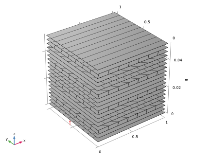
Modeling a composite laminate as a layered shell requires a surface geometry, in general referred to as a base surface, and a Layered Material node which adds an extra dimension (1D) to the base surface geometry in the surface normal direction. You can use the Layered Material functionality to model several layers stacked on top of each other having different thicknesses, material properties, and fiber orientations. You can optionally specify the interface materials between the layers, and control the number of through-thickness mesh elements for each layer.
The third direction for the selected coordinate system in the Single Layer Material, Layered Material Link, or Layered Material Stack represents the normal direction of the Layered Shell or Shell physics. This is also the direction in which the layer stacking is interpreted from bottom to top, and therefore, it is crucial to know it during modeling. There are two ways to achieve this:
-
Using physics symbols: Go to the physics settings, find the Physics Symbols section, and select the Enable physics symbols checkbox. Then go to the material feature, for instance, Linear Elastic Material, to see the normal direction represented by green arrows in the geometry.
-
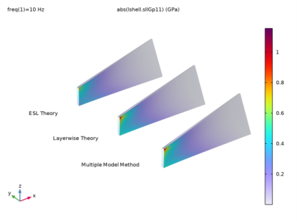
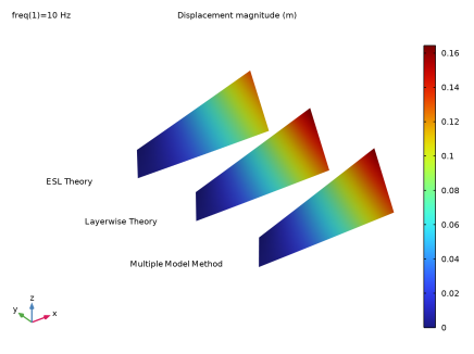
To model composites you can use two approaches: You can use either the Layered Shell interface, that uses the layerwise theory, or the Linear Elastic Material, Layered node in the Shell interface, that uses the Equivalent Single Layer (ESL) theory.
The multiple model method combines the aforementioned modeling approaches, and in order to combine the Layered Shell and Shell interfaces in the thickness direction, a Layered Shell-Shell Connection multiphysics coupling must be used. You must also use the Layered Material Stack node for the through-thickness coupling between the interfaces.
In a situation where Layered Shell and Shell interfaces are coupled in-plane, you must use a Layered Shell-Structural Transition multiphysics coupling. Here, the same Single Layer Material, Layered Material Link or Layered Material Stack node must be used in both interfaces. This modeling approach is also a multiple model method.
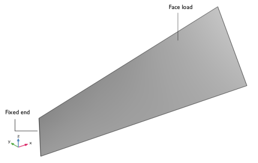
It is not advised to use the Layered Shell interface for discontinuous layers, as it can create problems in fold-line constraints. No fold-lines exist in the present model, hence the Layered Shell interface used to model the PVC foam and the carbon–epoxy layers.
Reference
1. J.N. Reddy, Mechanics of Laminated Composite Plates and Shells: Theory and Analysis, 2nd ed., CRC Press, 2004.
Application Library path: Composite_Materials_Module/Tutorials/composite_blade_multiple_model_method
Modeling Instructions
From the File menu, choose New.
New
In the New window, click  Model Wizard.
Model Wizard
1
In the Model Wizard window, click  3D.
2
In the Select Physics tree, select Structural Mechanics > Layered Shell (lshell).
3
Click Add.
4
In the Select Physics tree, select Structural Mechanics > Shell (shell).
5
Click Add.
6
Click  Study.
7
In the Select Study tree, select General Studies > Eigenfrequency.
8
Global Definitions
Parameters 1
1
In the Model Builder window, under Global Definitions click Parameters 1.
2
In the Settings window for Parameters, locate the Parameters section.
3
Material: Carbon–Epoxy
1
In the Model Builder window, under Global Definitions right-click Materials and choose Blank Material.
2
In the Settings window for Material, type Material: Carbon-Epoxy in the Label text field.
Layered Material: CE-[0]
1
Right-click Materials and choose Layered Material.
2
In the Settings window for Layered Material, type Layered Material: CE-[0] in the Label text field.
3
Locate the Layer Definition section. In the table, enter the following settings:
Material: Glass–Vinylester
1
Right-click Materials and choose Blank Material.
2
In the Settings window for Material, type Material: Glass-Vinylester in the Label text field.
Layered Material: GV-[0/45/-45/90]_s
1
Right-click Materials and choose Layered Material.
2
In the Settings window for Layered Material, type Layered Material: GV-[0/45/-45/90]_s in the Label text field.
3
Locate the Layer Definition section. In the table, enter the following settings:
4
Add six additional layers so that the material has a total of eight layers.
5
6
Click to expand the Preview Plot Settings section. In the Thickness-to-width ratio text field, type 0.6.
7
Locate the Layer Definition section. Click Layer Stack Preview in the upper-right corner of the section.
Material: PVC Foam
1
Right-click Materials and choose Blank Material.
2
In the Settings window for Material, type Material: PVC Foam in the Label text field.
Layered Material: PF-[0]
1
Right-click Materials and choose Layered Material.
2
In the Settings window for Layered Material, type Layered Material: PF-[0] in the Label text field.
3
Locate the Layer Definition section. In the table, enter the following settings:
Geometry 1
Work Plane 1 (wp1)
1
In the Geometry toolbar, click  Work Plane.
2
In the Settings window for Work Plane, locate the Plane Definition section.
3
From the Plane list, choose yz-plane.
4
Click  Go to Plane Geometry.
Work Plane 1 (wp1) > Line Segment 1 (ls1)
1
In the Work Plane toolbar, click  More Primitives and choose Line Segment.
2
In the Settings window for Line Segment, locate the Starting Point section.
3
From the Specify list, choose Coordinates.
4
Locate the Endpoint section. From the Specify list, choose Coordinates.
5
In the yw text field, type 0.4.
Extrude 1 (ext1)
1
In the Model Builder window, right-click Geometry 1 and choose Extrude.
2
In the Settings window for Extrude, locate the Distances section.
3
4
Select the Reverse direction checkbox.
5
Click to expand the Scales section. In the table, enter the following settings:
6
Click to expand the Twist Angles section. In the table, enter the following settings:
7
Click  Build All Objects.
8
Click the  Zoom Extents button in the Graphics toolbar.
9
Click the  Show Grid button in the Graphics toolbar.
Definitions
Boundary System 1 (sys1)
1
In the Model Builder window, expand the Component 1 (comp1) > Definitions node, then click Boundary System 1 (sys1).
2
In the Settings window for Boundary System, locate the Settings section.
3
Find the Coordinate names subsection. From the Axis list, choose x.
Materials
The laminate is modeled using a Layered Material Stack node. Multiple layered material links are added to demonstrate the multiple model method.
Layered Material Stack 1 (stlmat1)
In the Model Builder window, under Component 1 (comp1) right-click Materials and choose Layers > Layered Material Stack.
Carbon–Epoxy-1 [0]
In the Settings window for Layered Material Link, type Carbon-Epoxy-1 [0] in the Label text field.
Glass–Vinylester-1 [0/45/-45/90]_s
1
Right-click Carbon–Epoxy-1 [0] and choose Duplicate.
2
In the Settings window for Layered Material Link, type Glass-Vinylester-1 [0/45/-45/90]_s in the Label text field.
3
Locate the Link Settings section. From the Material list, choose Layered Material: GV-[0/45/-45/90]_s (lmat2).
PVC Foam [0]
1
Right-click Glass–Vinylester-1 [0/45/-45/90]_s and choose Duplicate.
2
In the Settings window for Layered Material Link, type PVC Foam [0] in the Label text field.
3
Locate the Link Settings section. From the Material list, choose Layered Material: PF-[0] (lmat3).
Glass–Vinylester-2 [0/45/-45/90]_s
1
Right-click PVC Foam [0] and choose Duplicate.
2
In the Settings window for Layered Material Link, type Glass-Vinylester-2 [0/45/-45/90]_s in the Label text field.
3
Locate the Link Settings section. From the Material list, choose Layered Material: GV-[0/45/-45/90]_s (lmat2).
Carbon–Epoxy-2 [0]
1
Right-click Glass–Vinylester-2 [0/45/-45/90]_s and choose Duplicate.
2
In the Settings window for Layered Material Link, type Carbon-Epoxy-2 [0] in the Label text field.
3
Locate the Link Settings section. From the Material list, choose Layered Material: CE-[0] (lmat1).
Layered Material Stack 1 (stlmat1)
1
In the Model Builder window, click Layered Material Stack 1 (stlmat1).
2
In the Settings window for Layered Material Stack, click to expand the Preview Plot Settings section.
3
In the Thickness-to-width ratio text field, type 0.4.
4
Click Layer Cross-Section Preview in the upper-right corner of the Layered Material Settings section. From the menu, choose Layer Cross-Section Preview to enable the through-thickness view of the laminated material, as in Figure 2.
5
Click Section_bar in the upper-right corner of the Layered Material Settings section. From the menu, choose Layer Stack Preview.
6
Locate the Preview Plot Settings section. In the Thickness-to-width ratio text field, type 1.
7
Click Layer Stack Preview in the upper-right corner of the Layered Material Settings section. From the menu, choose Layer Stack Preview to show the stacking sequence, including the fiber orientation, as in Figure 3.
Modeling Instructions (Frequency and Eigenfrequency Analysis Using the Multiple Model Method)
This section describes how to model a composite blade using the multiple model method. To this end, you will use one Layered Shell and two Shell interfaces.
Layered Shell (Multiple Model Method)
1
In the Model Builder window, under Component 1 (comp1) click Layered Shell (lshell).
2
In the Settings window for Layered Shell, type Layered Shell (Multiple Model Method) in the Label text field.
Add the material properties for the carbon-epoxy, the glass-vinylester, and the PVC foam.
3
Locate the Shell Properties section. Clear the Use all layers checkbox.
4
Click  Clear All.
5
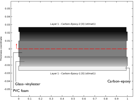
In the Selection table, select the checkboxes for Layer 1 - Carbon–Epoxy-1 [0], Layer 1 - PVC Foam [0], and Layer 1 - Carbon–Epoxy-2 [0].
Linear Elastic Material 1
1
In the Model Builder window, under Component 1 (comp1) > Layered Shell (Multiple Model Method) (lshell) click Linear Elastic Material 1.
2
In the Settings window for Linear Elastic Material, locate the Linear Elastic Material section.
3
Select the Transversely isotropic checkbox.
Fixed Constraint 1
1
In the Physics toolbar, click  Edges and choose Fixed Constraint.
2
3
In the Settings window for Fixed Constraint, locate the Shell Properties section.
4
Select the Use all layers checkbox.
Face Load, Pressure
1
In the Physics toolbar, click  Boundaries and choose Face Load.
2
In the Settings window for Face Load, type Face Load, Pressure in the Label text field.
3
4
Locate the Interface Selection section. From the Apply to list, choose Top interface.
5
Locate the Force section. From the Load type list, choose Pressure.
6
In the p text field, type p0*exp(-j*mn*atan2(Y,X)).
Shell 1 (Multiple Model Method)
1
In the Model Builder window, under Component 1 (comp1) click Shell (shell).
2
In the Settings window for Shell, type Shell 1 (Multiple Model Method) in the Label text field.
3
Click the  Show More Options button in the Model Builder toolbar.
4
In the Show More Options dialog, in the tree, select the checkbox for the node Physics > Advanced Physics Options.
5
6
In the Settings window for Shell, click to expand the Advanced Settings section.
7
Clear the Use MITC interpolation checkbox.
Linear Elastic Material, Layered 1
1
In the Physics toolbar, click  Boundaries and choose Linear Elastic Material, Layered.
2
3
In the Settings window for Linear Elastic Material, Layered, locate the Shell Properties section.
4
Clear the Use all layers checkbox.
5
From the Stack member list, choose Glass–Vinylester-1 [0/45/-45/90]_s (stlmat1.stllmat2).
6
Locate the Linear Elastic Material section. From the Material symmetry list, choose Orthotropic.
7
Select the Transversely isotropic checkbox.
8
Click to expand the Shear Correction Factor section. From the list, choose User defined.
Fixed Constraint 1
1
In the Physics toolbar, click  Edges and choose Fixed Constraint.
2
3
In the Model Builder window, right-click Shell 1 (Multiple Model Method) (shell) and choose Copy.
Shell 2 (Multiple Model Method)
1
In the Model Builder window, right-click Component 1 (comp1) and choose Paste Shell.
2
In the Messages from Paste dialog, click OK.
3
In the Settings window for Shell, type Shell 2 (Multiple Model Method) in the Label text field.
Linear Elastic Material, Layered 1
1
In the Model Builder window, expand the Component 1 (comp1) > Shell 2 (Multiple Model Method) (shell2) node, then click Linear Elastic Material, Layered 1.
2
In the Settings window for Linear Elastic Material, Layered, locate the Shell Properties section.
3
From the Stack member list, choose Glass–Vinylester-2 [0/45/-45/90]_s (stlmat1.stllmat4).
Global Definitions
Material: Carbon–Epoxy (mat1)
1
In the Model Builder window, under Global Definitions > Materials click Material: Carbon–Epoxy (mat1).
2
In the Settings window for Material, locate the Material Contents section.
3
Material: Glass–Vinylester (mat2)
1
In the Model Builder window, click Material: Glass–Vinylester (mat2).
2
In the Settings window for Material, locate the Material Contents section.
3
Material: PVC Foam (mat3)
1
In the Model Builder window, click Material: PVC Foam (mat3).
2
In the Settings window for Material, locate the Material Contents section.
3
Multiphysics
Layered Shell–Shell Connection 1 (lssh1)
In the Physics toolbar, click  Multiphysics Couplings and choose Boundary > Layered Shell–Shell Connection.
Layered Shell–Shell Connection 2 (lssh2)
1
Right-click Layered Shell–Shell Connection 1 (lssh1) and choose Duplicate.
2
In the Settings window for Layered Shell–Shell Connection, locate the Coupled Interfaces section.
3
From the Shell list, choose Shell 2 (Multiple Model Method) (shell2).
Mesh 1
In the Model Builder window, under Component 1 (comp1) right-click Mesh 1 and choose Build All.
Study: Eigenfrequency (Multiple Model Method)
Switch off the generation of default plots in every study. We will use customized plots for comparison purposes.
1
In the Model Builder window, click Study 1.
2
In the Settings window for Study, type Study: Eigenfrequency (Multiple Model Method) in the Label text field.
3
Locate the Study Settings section. Clear the Generate default plots checkbox.
Solution 1 (sol1)
In the Study toolbar, click  Show Default Solver.
Solution 1 (sol1)
1
In the Model Builder window, expand the Study: Eigenfrequency (Multiple Model Method) > Solver Configurations > Solution 1 (sol1) node, then click Eigenvalue Solver 1.
2
In the Settings window for Eigenvalue Solver, locate the Output section.
3
From the Scaling of eigenvectors list, choose RMS.
4
In the Study toolbar, click  Compute.
Results
Layered Material 1
1
In the Model Builder window, expand the Results node.
2
Right-click Results > Datasets and choose More Datasets > Layered Material.
Mode Shapes (Multiple Model Method)
1
In the Results toolbar, click  3D Plot Group.
2
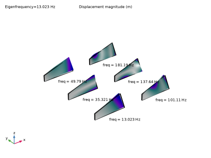
In the Settings window for 3D Plot Group, type Mode Shapes (Multiple Model Method) in the Label text field.
3
Locate the Data section. From the Dataset list, choose Layered Material 1.
4
Locate the Color Legend section. Clear the Show legends checkbox.
5
Click to expand the Plot Array section. From the Array type list, choose Square.
6
In the Relative row padding text field, type 1.
7
In the Relative column padding text field, type 0.6.
Surface 1
1
Right-click Mode Shapes (Multiple Model Method) and choose Surface.
2
In the Settings window for Surface, locate the Coloring and Style section.
3
From the Color table list, choose AuroraAustralis.
Deformation 1
Right-click Surface 1 and choose Deformation.
Solution Array 1
1
In the Model Builder window, right-click Surface 1 and choose Solution Array.
2
In the Settings window for Solution Array, locate the Plot Array section.
3
From the Array shape list, choose Square.
4
From the Order list, choose Column-major.
Surface 2
1
Right-click Surface 1 and choose Duplicate.
2
In the Settings window for Surface, locate the Expression section.
3
In the Expression text field, type shell.disp.
4
Click to expand the Title section. From the Title type list, choose None.
5
Click to expand the Inherit Style section. From the Plot list, choose Surface 1.
6
Click to expand the Plot Array section. Select the Manual indexing checkbox.
Deformation 1
1
In the Model Builder window, expand the Surface 2 node, then click Deformation 1.
2
In the Settings window for Deformation, locate the Expression section.
3
In the x-component text field, type u2.
4
In the y-component text field, type v2.
5
In the z-component text field, type w2.
Surface 3
1
In the Model Builder window, under Results > Mode Shapes (Multiple Model Method) right-click Surface 2 and choose Duplicate.
2
In the Settings window for Surface, locate the Expression section.
3
In the Expression text field, type shell2.disp.
Deformation 1
1
In the Model Builder window, expand the Surface 3 node, then click Deformation 1.
2
In the Settings window for Deformation, locate the Expression section.
3
In the x-component text field, type u3.
4
In the y-component text field, type v3.
5
In the z-component text field, type w3.
Annotation 1
1
In the Model Builder window, right-click Mode Shapes (Multiple Model Method) and choose Annotation.
2
In the Settings window for Annotation, locate the Annotation section.
3
In the Text text field, type freq = eval(freq,Hz,5) Hz.
4
From the Geometry level list, choose Global.
5
Locate the Position section. In the x text field, type 0.7.
6
In the y text field, type -0.1.
7
Locate the Coloring and Style section. Clear the Show point checkbox.
8
Click to expand the Plot Array section. Select the Manual indexing checkbox.
Solution Array 1
In the Model Builder window, under Results > Mode Shapes (Multiple Model Method) > Surface 1 right-click Solution Array 1 and choose Copy.
Solution Array 1
In the Model Builder window, right-click Annotation 1 and choose Paste Solution Array.
Mode Shapes (Multiple Model Method)
1
In the Settings window for 3D Plot Group, locate the Plot Settings section.
2
From the View list, choose New view.
3
In the Mode Shapes (Multiple Model Method) toolbar, click  Plot.
Add Study
1
In the Home toolbar, click  Add Study to open the Add Study window.
2
Go to the Add Study window.
3
Find the Studies subsection. In the Select Study tree, select General Studies > Frequency Domain.
4
Click the Add Study button in the window toolbar.
5
In the Home toolbar, click  Add Study to close the Add Study window.
Study 2
Step 1: Frequency Domain
1
In the Settings window for Frequency Domain, locate the Study Settings section.
2
In the Frequencies text field, type 10.
3
In the Model Builder window, click Study 2.
4
In the Settings window for Study, type Study: Frequency (Multiple Model Method) in the Label text field.
5
Locate the Study Settings section. Clear the Generate default plots checkbox.
6
In the Study toolbar, click  Compute.
Results
Layered Material 2
1
In the Results toolbar, click  More Datasets and choose Layered Material.
2
In the Settings window for Layered Material, locate the Data section.
3
From the Dataset list, choose Study: Frequency (Multiple Model Method)/Solution 2 (sol2).
Stress
1
In the Results toolbar, click  3D Plot Group.
2
In the Settings window for 3D Plot Group, type Stress in the Label text field.
3
Locate the Data section. From the Dataset list, choose Layered Material 2.
4
Locate the Plot Settings section. From the View list, choose New view.
5
In the Stress toolbar, click  Plot.
This generates a dedicated view for the plot.
6
Clear the Plot dataset edges checkbox.
Surface 1
1
Right-click Stress and choose Surface.
2
In the Settings window for Surface, locate the Expression section.
3
In the Expression text field, type abs(lshell.sllGp11).
4
From the Unit list, choose GPa.
5
Locate the Coloring and Style section. From the Color table list, choose Prism.
Deformation 1
Right-click Surface 1 and choose Deformation.
Surface 2
1
In the Model Builder window, under Results > Stress right-click Surface 1 and choose Duplicate.
2
In the Settings window for Surface, locate the Title section.
3
From the Title type list, choose None.
4
Locate the Inherit Style section. From the Plot list, choose Surface 1.
Deformation 1
1
In the Model Builder window, expand the Surface 2 node, then click Deformation 1.
2
In the Settings window for Deformation, locate the Expression section.
3
In the x-component text field, type u2.
4
In the y-component text field, type v2.
5
In the z-component text field, type w2.
Surface 2
1
In the Model Builder window, click Surface 2.
2
In the Settings window for Surface, locate the Expression section.
3
In the Expression text field, type abs(shell.sllGp11).
Surface 3
Right-click Results > Stress > Surface 2 and choose Duplicate.
Deformation 1
1
In the Model Builder window, expand the Surface 3 node, then click Deformation 1.
2
In the Settings window for Deformation, locate the Expression section.
3
In the x-component text field, type u3.
4
In the y-component text field, type v3.
5
In the z-component text field, type w3.
Surface 3
1
In the Model Builder window, click Surface 3.
2
In the Settings window for Surface, locate the Expression section.
3
In the Expression text field, type abs(shell2.sllGp11).
Stress
1
In the Model Builder window, click Stress.
2
In the Stress toolbar, click  Plot.
Displacement, Slice
1
In the Results toolbar, click  3D Plot Group.
2
In the Settings window for 3D Plot Group, type Displacement, Slice in the Label text field.
3
Locate the Data section. From the Dataset list, choose Study: Frequency (Multiple Model Method)/Solution 2 (sol2).
4
Locate the Plot Settings section. From the View list, choose View 3D 5.
5
Clear the Plot dataset edges checkbox.
Layered Material Slice 1
1
In the Displacement, Slice toolbar, click  More Plots and choose Layered Material Slice.
2
In the Settings window for Layered Material Slice, locate the Through-Thickness Location section.
3
From the Location definition list, choose Relative.
4
In the Local z-coordinate [-1,1] text field, type 1.
Displacement, Slice
1
In the Model Builder window, click Displacement, Slice.
2
In the Displacement, Slice toolbar, click  Plot.
Modeling Instructions (Frequency and Eigenfrequency Analysis Using the Layerwise (LW) Theory)
This section describes how to model a composite blade using the Layered Shell interface based on the layerwise theory.
Layered Shell (Multiple Model Method) (lshell)
In the Model Builder window, under Component 1 (comp1) right-click Layered Shell (Multiple Model Method) (lshell) and choose Copy.
Layered Shell (Layerwise Theory)
1
In the Model Builder window, right-click Component 1 (comp1) and choose Paste Layered Shell.
2
In the Messages from Paste dialog, click OK.
3
In the Settings window for Layered Shell, type Layered Shell (Layerwise Theory) in the Label text field.
4
Locate the Shell Properties section. Select the Use all layers checkbox.
Add Study
1
In the Home toolbar, click  Add Study to open the Add Study window.
2
Go to the Add Study window.
3
Find the Studies subsection. In the Select Study tree, select General Studies > Eigenfrequency.
4
Click the Add Study button in the window toolbar.
5
In the Home toolbar, click  Add Study to close the Add Study window.
Study: Eigenfrequency (Layerwise Theory)
1
In the Settings window for Study, type Study: Eigenfrequency (Layerwise Theory) in the Label text field.
2
Locate the Study Settings section. Clear the Generate default plots checkbox.
Step 1: Eigenfrequency
1
In the Model Builder window, under Study: Eigenfrequency (Layerwise Theory) click Step 1: Eigenfrequency.
2
In the Settings window for Eigenfrequency, locate the Physics and Variables Selection section.
3
Select the Modify model configuration for study step checkbox.
4
In the tree, select Component 1 (comp1) > Layered Shell (Multiple Model Method) (lshell), Component 1 (comp1) > Shell 1 (Multiple Model Method) (shell), and Component 1 (comp1) > Shell 2 (Multiple Model Method) (shell2).
5
Click  Disable in Model.
6
In the tree, select Component 1 (comp1) > Multiphysics > Layered Shell–Shell Connection 1 (lssh1) and Component 1 (comp1) > Multiphysics > Layered Shell–Shell Connection 2 (lssh2).
7
Click  Disable in Model.
Solution 3 (sol3)
In the Study toolbar, click  Show Default Solver.
Solution 3 (sol3)
1
In the Model Builder window, expand the Study: Eigenfrequency (Layerwise Theory) > Solver Configurations > Solution 3 (sol3) node, then click Eigenvalue Solver 1.
2
In the Settings window for Eigenvalue Solver, locate the Output section.
3
From the Scaling of eigenvectors list, choose RMS.
4
In the Study toolbar, click  Compute.
Results
Layered Material 3
1
In the Model Builder window, under Results > Datasets right-click Layered Material 1 and choose Duplicate.
2
In the Settings window for Layered Material, locate the Data section.
3
From the Dataset list, choose Study: Eigenfrequency (Layerwise Theory)/Solution 3 (sol3).
Mode Shapes (Layerwise Theory)
1
In the Model Builder window, right-click Mode Shapes (Multiple Model Method) and choose Duplicate.
2
In the Settings window for 3D Plot Group, type Mode Shapes (Layerwise Theory) in the Label text field.
3
Locate the Data section. From the Dataset list, choose None.
4
In the Model Builder window, expand the Mode Shapes (Layerwise Theory) node.
Surface 2, Surface 3
1
In the Model Builder window, under Results > Mode Shapes (Layerwise Theory), Ctrl-click to select Surface 2 and Surface 3.
2
Surface 1
1
In the Model Builder window, under Results > Mode Shapes (Layerwise Theory) click Surface 1.
2
In the Settings window for Surface, locate the Expression section.
3
In the Expression text field, type lshell2.disp.
Deformation 1
1
In the Model Builder window, click Deformation 1.
2
In the Settings window for Deformation, locate the Expression section.
3
In the x-component text field, type u4.
4
In the y-component text field, type v4.
5
In the z-component text field, type w4.
Mode Shapes (Layerwise Theory)
1
In the Model Builder window, under Results click Mode Shapes (Layerwise Theory).
2
In the Settings window for 3D Plot Group, locate the Data section.
3
From the Dataset list, choose Layered Material 3.
4
Click the  Zoom Extents button in the Graphics toolbar.
5
In the Mode Shapes (Layerwise Theory) toolbar, click  Plot.
Add Study
1
In the Home toolbar, click  Add Study to open the Add Study window.
2
Go to the Add Study window.
3
Find the Studies subsection. In the Select Study tree, select General Studies > Frequency Domain.
4
Click the Add Study button in the window toolbar.
5
In the Home toolbar, click  Add Study to close the Add Study window.
Study 4
Step 1: Frequency Domain
1
In the Settings window for Frequency Domain, locate the Study Settings section.
2
In the Frequencies text field, type 10.
3
Locate the Physics and Variables Selection section. Select the Modify model configuration for study step checkbox.
4
In the tree, select Component 1 (comp1) > Layered Shell (Multiple Model Method) (lshell), Component 1 (comp1) > Shell 1 (Multiple Model Method) (shell), and Component 1 (comp1) > Shell 2 (Multiple Model Method) (shell2).
5
Click  Disable in Model.
6
In the tree, select Component 1 (comp1) > Multiphysics > Layered Shell–Shell Connection 1 (lssh1) and Component 1 (comp1) > Multiphysics > Layered Shell–Shell Connection 2 (lssh2).
7
Click  Disable in Model.
8
In the Model Builder window, click Study 4.
9
In the Settings window for Study, type Study: Frequency (Layerwise Theory) in the Label text field.
10
Locate the Study Settings section. Clear the Generate default plots checkbox.
11
In the Study toolbar, click  Compute.
Results
Layered Material 4
1
In the Model Builder window, under Results > Datasets right-click Layered Material 2 and choose Duplicate.
2
In the Settings window for Layered Material, locate the Data section.
3
From the Dataset list, choose Study: Frequency (Layerwise Theory)/Solution 4 (sol4).
Stress
1
In the Model Builder window, under Results click Stress.
2
In the Settings window for 3D Plot Group, locate the Plot Array section.
3
From the Array type list, choose Linear.
4
From the Array axis list, choose y.
5
In the Relative padding text field, type 2.
Surface 2
1
In the Model Builder window, click Surface 2.
2
In the Settings window for Surface, locate the Plot Array section.
3
Select the Manual indexing checkbox.
Surface 3
1
In the Model Builder window, click Surface 3.
2
In the Settings window for Surface, locate the Plot Array section.
3
Select the Manual indexing checkbox.
Surface 4
1
Right-click Results > Stress > Surface 3 and choose Duplicate.
2
In the Settings window for Surface, locate the Data section.
3
From the Dataset list, choose Layered Material 4.
4
Locate the Expression section. In the Expression text field, type abs(lshell2.sllGp11).
5
Locate the Plot Array section. In the Index text field, type 1.
Deformation 1
1
In the Model Builder window, expand the Surface 4 node, then click Deformation 1.
2
In the Settings window for Deformation, locate the Expression section.
3
In the x-component text field, type u4.
4
In the y-component text field, type v4.
5
In the z-component text field, type w4.
Stress
1
In the Model Builder window, under Results click Stress.
2
In the Stress toolbar, click  Plot.
Displacement, Slice
1
In the Model Builder window, click Displacement, Slice.
2
In the Settings window for 3D Plot Group, locate the Plot Array section.
3
From the Array type list, choose Linear.
4
From the Array axis list, choose y.
5
In the Relative padding text field, type 2.
Layered Material Slice 2
1
In the Model Builder window, under Results > Displacement, Slice right-click Layered Material Slice 1 and choose Duplicate.
2
In the Settings window for Layered Material Slice, locate the Data section.
3
From the Dataset list, choose Study: Frequency (Layerwise Theory)/Solution 4 (sol4).
4
Locate the Expression section. In the Expression text field, type lshell2.disp.
5
Click to expand the Title section. From the Title type list, choose None.
6
Click to expand the Inherit Style section. From the Plot list, choose Layered Material Slice 1.
7
In the Displacement, Slice toolbar, click  Plot.
Modeling Instructions (Frequency and Eigenfrequency Analysis using the Equivalent Single Layer (ESL) Theory)
This section describes how to model a composite blade using the Shell interface based on the equivalent single layer (ESL) theory.
Shell 1 (Multiple Model Method) (shell)
In the Model Builder window, under Component 1 (comp1) right-click Shell 1 (Multiple Model Method) (shell) and choose Copy.
Shell (ESL Theory)
1
In the Model Builder window, right-click Component 1 (comp1) and choose Paste Shell.
2
In the Messages from Paste dialog, click OK.
3
In the Settings window for Shell, type Shell (ESL Theory) in the Label text field.
Linear Elastic Material, Layered 1
1
In the Model Builder window, expand the Component 1 (comp1) > Shell (ESL Theory) (shell3) node, then click Linear Elastic Material, Layered 1.
2
In the Settings window for Linear Elastic Material, Layered, locate the Shell Properties section.
3
Select the Use all layers checkbox.
Face Load, Pressure
1
In the Physics toolbar, click  Boundaries and choose Face Load.
2
In the Settings window for Face Load, type Face Load, Pressure in the Label text field.
3
4
Locate the Through-Thickness Location section. From the list, choose Top surface.
5
Locate the Force section. From the Load type list, choose Pressure.
6
In the p text field, type p0*exp(-j*mn*atan2(Y,X)).
Add Study
1
In the Home toolbar, click  Add Study to open the Add Study window.
2
Go to the Add Study window.
3
Find the Studies subsection. In the Select Study tree, select General Studies > Eigenfrequency.
4
Click the Add Study button in the window toolbar.
5
In the Home toolbar, click  Add Study to close the Add Study window.
Study: Eigenfrequency (ESL Theory)
1
In the Settings window for Study, type Study: Eigenfrequency (ESL Theory) in the Label text field.
2
Locate the Study Settings section. Clear the Generate default plots checkbox.
Step 1: Eigenfrequency
1
In the Model Builder window, under Study: Eigenfrequency (ESL Theory) click Step 1: Eigenfrequency.
2
In the Settings window for Eigenfrequency, locate the Physics and Variables Selection section.
3
Select the Modify model configuration for study step checkbox.
4
In the tree, select Component 1 (comp1) > Layered Shell (Multiple Model Method) (lshell), Component 1 (comp1) > Shell 1 (Multiple Model Method) (shell), Component 1 (comp1) > Shell 2 (Multiple Model Method) (shell2), and Component 1 (comp1) > Layered Shell (Layerwise Theory) (lshell2).
5
Click  Disable in Model.
6
In the tree, select Component 1 (comp1) > Multiphysics > Layered Shell–Shell Connection 1 (lssh1) and Component 1 (comp1) > Multiphysics > Layered Shell–Shell Connection 2 (lssh2).
7
Click  Disable in Model.
Solution 5 (sol5)
In the Study toolbar, click  Show Default Solver.
Solution 5 (sol5)
1
In the Model Builder window, expand the Study: Eigenfrequency (ESL Theory) > Solver Configurations > Solution 5 (sol5) node, then click Eigenvalue Solver 1.
2
In the Settings window for Eigenvalue Solver, locate the Output section.
3
From the Scaling of eigenvectors list, choose RMS.
4
In the Study toolbar, click  Compute.
Results
Layered Material 5
1
In the Model Builder window, under Results > Datasets right-click Layered Material 1 and choose Duplicate.
2
In the Settings window for Layered Material, locate the Data section.
3
From the Dataset list, choose Study: Eigenfrequency (ESL Theory)/Solution 5 (sol5).
Mode Shapes (ESL Theory)
1
In the Model Builder window, right-click Mode Shapes (Layerwise Theory) and choose Duplicate.
2
In the Settings window for 3D Plot Group, type Mode Shapes (ESL Theory) in the Label text field.
3
Locate the Data section. From the Dataset list, choose None.
Surface 1
1
In the Model Builder window, expand the Mode Shapes (ESL Theory) node, then click Surface 1.
2
In the Settings window for Surface, locate the Expression section.
3
In the Expression text field, type shell3.disp.
Deformation 1
1
In the Model Builder window, click Deformation 1.
2
In the Settings window for Deformation, locate the Expression section.
3
In the x-component text field, type u5.
4
In the y-component text field, type v5.
5
In the z-component text field, type w5.
Mode Shapes (ESL Theory)
1
In the Model Builder window, under Results click Mode Shapes (ESL Theory).
2
In the Settings window for 3D Plot Group, locate the Data section.
3
From the Dataset list, choose Layered Material 5.
4
Click the  Zoom Extents button in the Graphics toolbar.
5
In the Mode Shapes (ESL Theory) toolbar, click  Plot.
Add Study
1
In the Home toolbar, click  Add Study to open the Add Study window.
2
Go to the Add Study window.
3
Find the Studies subsection. In the Select Study tree, select General Studies > Frequency Domain.
4
Click the Add Study button in the window toolbar.
5
In the Home toolbar, click  Add Study to close the Add Study window.
Study 6
Step 1: Frequency Domain
1
In the Settings window for Frequency Domain, locate the Study Settings section.
2
In the Frequencies text field, type 10.
3
Locate the Physics and Variables Selection section. Select the Modify model configuration for study step checkbox.
4
In the tree, select Component 1 (comp1) > Layered Shell (Multiple Model Method) (lshell), Component 1 (comp1) > Shell 1 (Multiple Model Method) (shell), Component 1 (comp1) > Shell 2 (Multiple Model Method) (shell2), and Component 1 (comp1) > Layered Shell (Layerwise Theory) (lshell2).
5
Click  Disable in Model.
6
In the tree, select Component 1 (comp1) > Multiphysics > Layered Shell–Shell Connection 1 (lssh1) and Component 1 (comp1) > Multiphysics > Layered Shell–Shell Connection 2 (lssh2).
7
Click  Disable in Model.
8
In the Model Builder window, click Study 6.
9
In the Settings window for Study, type Study: Frequency (ESL Theory) in the Label text field.
10
Locate the Study Settings section. Clear the Generate default plots checkbox.
11
In the Study toolbar, click  Compute.
Results
Layered Material 6
1
In the Model Builder window, under Results > Datasets right-click Layered Material 4 and choose Duplicate.
2
In the Settings window for Layered Material, locate the Data section.
3
From the Dataset list, choose Study: Frequency (ESL Theory)/Solution 6 (sol6).
Surface 5
1
In the Model Builder window, under Results > Stress right-click Surface 4 and choose Duplicate.
2
In the Settings window for Surface, locate the Data section.
3
From the Dataset list, choose Layered Material 6.
4
Locate the Expression section. In the Expression text field, type abs(shell3.sllGp11).
5
Locate the Plot Array section. In the Index text field, type 2.
Deformation 1
1
In the Model Builder window, expand the Surface 5 node, then click Deformation 1.
2
In the Settings window for Deformation, locate the Expression section.
3
In the x-component text field, type u5.
4
In the y-component text field, type v5.
5
In the z-component text field, type w5.
Stress
In the Model Builder window, under Results click Stress.
Table Annotation 1
1
In the Stress toolbar, click  More Plots and choose Table Annotation.
2
In the Settings window for Table Annotation, locate the Data section.
3
From the Source list, choose Local table.
4
5
Locate the Coloring and Style section. Clear the Show point checkbox.
6
From the Anchor point list, choose Lower middle.
7
In the Stress toolbar, click  Plot.
Layered Material Slice 3
1
In the Model Builder window, under Results > Displacement, Slice right-click Layered Material Slice 2 and choose Duplicate.
2
In the Settings window for Layered Material Slice, locate the Data section.
3
From the Dataset list, choose Study: Frequency (ESL Theory)/Solution 6 (sol6).
4
Locate the Expression section. In the Expression text field, type shell3.disp.
5
In the Displacement, Slice toolbar, click  Plot.
Table Annotation 1
In the Model Builder window, under Results > Stress right-click Table Annotation 1 and choose Copy.
Table Annotation 1
1
In the Model Builder window, right-click Displacement, Slice and choose Paste Table Annotation.
2
In the Displacement, Slice toolbar, click  Plot.
Comparison: Stress
1
In the Results toolbar, click  Evaluation Group.
2
In the Settings window for Evaluation Group, type Comparison: Stress in the Label text field.
3
Locate the Data section. From the Dataset list, choose Layered Material 2.
4
Click to expand the Format section. From the Include parameters list, choose Off.
Volume Maximum 1
1
Right-click Comparison: Stress and choose Maximum > Volume Maximum.
2
In the Settings window for Volume Maximum, locate the Expressions section.
3
Volume Maximum 2
1
Right-click Volume Maximum 1 and choose Duplicate.
2
In the Settings window for Volume Maximum, locate the Data section.
3
From the Dataset list, choose Layered Material 4.
4
Locate the Expressions section. In the table, enter the following settings:
Volume Maximum 3
1
Right-click Volume Maximum 2 and choose Duplicate.
2
In the Settings window for Volume Maximum, locate the Data section.
3
From the Dataset list, choose Layered Material 6.
4
Locate the Expressions section. In the table, enter the following settings:
5
In the Comparison: Stress toolbar, click  Evaluate.
Comparison: Maximum Displacement
1
In the Results toolbar, click  Evaluation Group.
2
In the Settings window for Evaluation Group, type Comparison: Maximum Displacement in the Label text field.
3
Locate the Data section. From the Dataset list, choose Layered Material 2.
4
Locate the Format section. From the Include parameters list, choose Off.
Volume Maximum 1
1
Right-click Comparison: Maximum Displacement and choose Maximum > Volume Maximum.
2
In the Settings window for Volume Maximum, locate the Expressions section.
3
Volume Maximum 2
1
Right-click Volume Maximum 1 and choose Duplicate.
2
In the Settings window for Volume Maximum, locate the Data section.
3
From the Dataset list, choose Layered Material 4.
4
Locate the Expressions section. In the table, enter the following settings:
Volume Maximum 3
1
Right-click Volume Maximum 2 and choose Duplicate.
2
In the Settings window for Volume Maximum, locate the Data section.
3
From the Dataset list, choose Layered Material 6.
4
Locate the Expressions section. In the table, enter the following settings:
5
In the Comparison: Maximum Displacement toolbar, click  Evaluate.
Comparison: Eigenfrequency
1
In the Results toolbar, click  Evaluation Group.
2
In the Settings window for Evaluation Group, type Comparison: Eigenfrequency in the Label text field.
3
Locate the Format section. From the Include parameters list, choose Off.
Global Evaluation 1
1
Right-click Comparison: Eigenfrequency and choose Global Evaluation.
2
In the Settings window for Global Evaluation, locate the Expressions section.
3
Global Evaluation 2
1
Right-click Global Evaluation 1 and choose Duplicate.
2
In the Settings window for Global Evaluation, locate the Data section.
3
From the Dataset list, choose Study: Eigenfrequency (Layerwise Theory)/Solution 3 (sol3).
Global Evaluation 3
1
Right-click Global Evaluation 2 and choose Duplicate.
2
In the Settings window for Global Evaluation, locate the Data section.
3
From the Dataset list, choose Study: Eigenfrequency (ESL Theory)/Solution 5 (sol5).
4
In the Comparison: Eigenfrequency toolbar, click  Evaluate.
In the first two studies, disable the newly added physics interfaces so that the studies can be run as originally configured.
Study: Eigenfrequency (Multiple Model Method)
Step 1: Eigenfrequency
1
In the Model Builder window, under Study: Eigenfrequency (Multiple Model Method) click Step 1: Eigenfrequency.
2
In the Settings window for Eigenfrequency, locate the Physics and Variables Selection section.
3
Select the Modify model configuration for study step checkbox.
4
In the tree, select Component 1 (comp1) > Layered Shell (Layerwise Theory) (lshell2) and Component 1 (comp1) > Shell (ESL Theory) (shell3).
5
Click  Disable in Model.
Study: Frequency (Multiple Model Method)
Step 1: Frequency Domain
1
In the Model Builder window, under Study: Frequency (Multiple Model Method) click Step 1: Frequency Domain.
2
In the Settings window for Frequency Domain, locate the Physics and Variables Selection section.
3
Select the Modify model configuration for study step checkbox.
4
In the tree, select Component 1 (comp1) > Layered Shell (Layerwise Theory) (lshell2) and Component 1 (comp1) > Shell (ESL Theory) (shell3).
5
Click  Disable in Model.
Study: Eigenfrequency (Layerwise Theory)
Step 1: Eigenfrequency
1
In the Model Builder window, under Study: Eigenfrequency (Layerwise Theory) click Step 1: Eigenfrequency.
2
In the Settings window for Eigenfrequency, locate the Physics and Variables Selection section.
3
In the tree, select Component 1 (comp1) > Shell (ESL Theory) (shell3).
4
Click  Disable in Model.
Study: Frequency (Layerwise Theory)
Step 1: Frequency Domain
1
In the Model Builder window, under Study: Frequency (Layerwise Theory) click Step 1: Frequency Domain.
2
In the Settings window for Frequency Domain, locate the Physics and Variables Selection section.
3
In the tree, select Component 1 (comp1) > Shell (ESL Theory) (shell3).
4
Click  Disable in Model.