PDF

Turbulent Aggregation of Nanoparticles
Introduction
Nanoparticles have become widely used in a range of applications. For example, in pharmaceuticals, particles on the nanoscale, such as nanocrystals, are often used as an effective means of drug delivery. Meanwhile in material sciences, nanoparticle coating is an increasingly common way to improve or change the properties of materials. Understanding the factors affecting the size of these particles is an important step to develop production processes that optimize the desired particle properties.
Model Definition
The term nanoparticle is used to describe particles on the nanoscale. This example models the turbulence-induced aggregation of nanoparticles in the size range of a few hundred nanometers in a beaker fitted with a square blade impeller to predict the size distribution of volume-equivalent spherical particle diameters. The model is set up with a 2D geometry describing the aggregation and movement of particles in a turbulent flow in the mixing plane (Figure 1). The entire domain is modeled as a rotating domain and the impeller is set to a rotational speed of 350 rpm.
Figure 1: Model geometry consisting of beaker with impeller.
The aggregation and flow is modeled with the Precipitation in Fluid Flow interface which couples a Size-Based Population Balance interface with a Single-Phase Fluid Flow interface. A k-ε model is used to account for the turbulent flow resulting from the mixing. In this example we exclude nucleation, growth and dissolution. Furthermore, the particles are also assumed small enough that breakage is negligible. The size distribution is modeled using a discretization of 20 size intervals, or bins, and a logarithmic interval distribution. For aggregation, logarithmic distributions are recommended. The aggregation contribution is modeled as (Ref. 1)
(1)
where L is the characteristic length and K is the aggregation kernel. This model assumes spherical particles in which case the characteristic length, L, is the diameter. The aggregation kernel is written with both a perikinetic and orthokinetic contribution. They describe the collisions due to Brownian motion and convective transport by the fluid respectively. They are given by (Ref. 2 and Ref. 3)
(2)
and
(3)
where Lj and Lk are the sizes of the two colliding particles. Furthermore, ν is the kinematic viscosity (m2/s), ε is the turbulent dissipation rate (m2/s3), ρ is the fluid density (kg/m3), kb is the Boltzmann constant (m2·kg/s2/K) and T is the temperature (K). The turbulent dissipation rate are solved for by the fluid flow interface. All particles are modeled as spherical where the size, L, is the diameter such that the system, in absence of nucleation, growth and dissolution, conserves the total particle volume. Assuming that the collision contributions (Equation 2 and Equation 3) are independent of each other and that the contributions are additive we can write
(4)
Here, W is the stability ratio. In this model a joint stability ratio is applied to both collision contributions. The stability ratio can range from 1 (no stabilization) to infinity (complete stabilization) and the specific value will depend on the system. Experiments are often required to find a suitable stability ratio. For example, if ions are adsorbed on the particle surface, the stability ratio will increase due to repelling electrostatic forces. Or, if the solution is supersaturated, it is possible for the crystal particles to form strong bonds using the solute, in the form of agglomerates, which gives a lower stability ratio. As was done by Schwarzer and Peukert in their model of barium sulfate nanoparticle aggregation (Ref. 2), we therefore test multiple stabilization ratios. Three weak stabilization scenarios are tested; W = 1, W = 10, and W = 100. A stabilization of W = 1 is equal to having no stabilization and is a common approximation for systems with negligible electrostatic forces.
At time t = 0, there is an arbitrary initial distribution of particles according to (modified from Ref. 4)
(5)
if L > Loffset and 0 otherwise. The constants N0, Lmean, and Loffset control the initial particle concentration, mean size, and starting point, respectively. The distribution can be seen in Figure 2.
Figure 2: Initial size distribution.
Results and Discussion
The velocity field can be seen in Figure 3. The largest velocity magnitude is located at the tips of the impeller. This is also where we will see the most orthokinetic aggregation.
Figure 3: Velocity field in the mixing plane.
Figure 4 shows the concentration of particles at 0.2, 0.4, 0.8, and 1.2 seconds after mixing has begun with w = 1. A more pronounced decrease in particle concentration is seen near the impeller where the turbulent dissipation rate is higher and the orthokinetic aggregation contribution is larger.
Figure 4: Particle concentration at different times for W = 1.
Figure 5 shows the average particle concentration and average size across the beaker. The average size can be seen to increase from 200 to 388, 229, and 203 nm while the particle concentration decreases from 6 × 1016 to 3.1 × 1015, 3.6 × 1016, and 5.7 × 1016 1/m3 for W = 1, 50, and 100, respectively.
Figure 5: Average particle size and number of particles.
Finally, Figure 6 shows the average size distribution at different times and stability ratios. The distribution is given at t = 0, 3, 6, and 10 seconds. For no stabilization, W = 1, the distribution almost immediately collapses into a smaller number of larger particles. This is also what was seen in Figure 5. The distribution for W = 10 flattens out at a slower rate. At this stability ratio the change in distribution profile is still pronounced. The combinations of sizes that can form a particles are fewer at smaller sizes, so for small particles we see that the death term (sink term) dominates. At the highest modeled stability ratio, W = 100, aggregation still takes place but the overall distribution profile does not change much over the modeled time span.
Figure 6: Size distribution at different times.
References
1. M. Ölander, Numerical Simulations for Battery Recycling, master’s thesis, KTH, Royal Institute of Technology, 2023.
2. H.C. Schwarzer and W. Peukert, “Combined experimental/numerical study on the precipitation of nanoparticles,” AICHE J., vol. 50, no. 12, pp. 3234–3247, 2004.
3. A. Raponi, S. Romano, G. Battaglia, A. Buffo, M. Vannie, A. Cipollina, and D. Marchisio, “Computational Modeling of Magnesium Hydroxide Precipitation and Kinetics Parameters Identification,” Cryst. Growth Des., vol. 23, no. 12, pp. 4748-4759, 2023.
4. W. Zhang, T. Przybycien, J.M. Breuer, and E. von Lieres, “Solving crystallization/precipitation population balance models in CADET, Part II: Size-based Smoluchowski coagulation and fragmentation equations in batch and continuous modes,” Comput. Chem. Eng., vol. 192, 2025.
Application Library path: Chemical_Reaction_Engineering_Module/Mixing_and_Separation/turbulent_aggregation
Modeling Instructions
From the File menu, choose New.
New
In the New window, click  Model Wizard.
Model Wizard
1
In the Model Wizard window, click  2D.
2
In the Select Physics tree, select Chemical Species Transport > Precipitation and Crystallization > Precipitation and Crystallization in Fluid Flow.
3
Click Add.
4
In the Added physics interfaces tree, select Transport of Diluted Species (tds).
5
Click Remove.
6
Global Definitions
Parameters 1
1
In the Model Builder window, under Global Definitions click Parameters 1.
2
In the Settings window for Parameters, locate the Parameters section.
3
Click  Load from File.
4
Definitions
Initial distribution
1
In the Definitions toolbar, click  Analytic.
2
In the Settings window for Analytic, type Initial distribution in the Label text field.
3
In the Function name text field, type initdist.
4
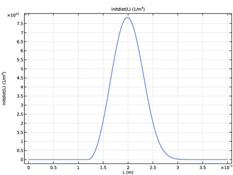
Locate the Definition section. In the Expression text field, type (L>L_offset)*3*(L-L_offset)^2*(N0)/((L_mean-L_offset)^3)*exp(-(L-L_offset)^3/(L_mean-L_offset)^3).
5
In the Arguments text field, type L.
6
Locate the Units section. In the Function text field, type 1/m^4.
7
8
Locate the Plot Parameters section. In the table, enter the following settings:
9
Geometry 1
Circle 1 (c1)
1
In the Geometry toolbar, click  Circle.
2
In the Settings window for Circle, locate the Size and Shape section.
3
In the Radius text field, type D_beaker/2.
Polygon 1 (pol1)
1
In the Geometry toolbar, click  Polygon.
2
In the Settings window for Polygon, locate the Coordinates section.
3
Click  Load from File.
4
Difference 1 (dif1)
1
In the Geometry toolbar, click  Booleans and Partitions and choose Difference.
2
3
In the Settings window for Difference, locate the Difference section.
4
Click to select the  Activate Selection toggle button for Objects to subtract.
5
6
Click  Build All Objects.
7
Click the  Zoom Extents button in the Graphics toolbar.
Add Material
1
In the Materials toolbar, click  Add Material to open the Add Material window.
2
Go to the Add Material window.
3
In the tree, select Built-in > Water, liquid.
4
Click the Add to Component button in the window toolbar.
Component 1 (comp1)
Rotating Domain 1
1
In the Physics toolbar, click  Moving Mesh and choose Rotating Domain.
2
In the Settings window for Rotating Domain, locate the Rotation section.
3
From the Rotation type list, choose Specified rotational velocity.
4
From the Rotational velocity expression list, choose General revolutions per time.
5
In the f text field, type rpm_impeller.
Laminar Flow (spf)
1
In the Model Builder window, under Component 1 (comp1) click Laminar Flow (spf).
2
In the Settings window for Laminar Flow, locate the Turbulence section.
3
From the Turbulence model type list, choose RANS-EVM.
Wall 1
1
In the Model Builder window, under Component 1 (comp1) > Turbulent Flow, k-ε (spf) click Wall 1.
2
In the Settings window for Wall, click to expand the Wall Movement section.
3
From the Translational velocity list, choose Zero (Fixed wall).
Wall 2
1
In the Physics toolbar, click  Boundaries and choose Wall.
2
Pressure Point Constraint 1
1
In the Physics toolbar, click  Points and choose Pressure Point Constraint.
2
Size-Based Population Balance (pbsb)
1
In the Model Builder window, under Component 1 (comp1) click Size-Based Population Balance (pbsb).
2
In the Settings window for Size-Based Population Balance, locate the Particle Properties section.
3
In the ρp text field, type rho_p.
4
Locate the Size Intervals section. From the Discretization list, choose Logarithmic.
5
In the I text field, type 20.
6
In the L0 text field, type L_offset.
7
In the LI text field, type 2000[nm].
8
Locate the Aggregation section. Select the Include checkbox.
9
In the K text field, type 1/W*(sqrt(pi/(15*8))*(pop.Lj+pop.Lk)^3*sqrt(max(ep,eps)/spf.nu)+2*k_B_const*T/(3*spf.nu*spf.rho)*(pop.Lj+pop.Lk)*(1/pop.Lj+1/pop.Lk)).
Initial Values 1
1
In the Model Builder window, under Component 1 (comp1) > Size-Based Population Balance (pbsb) click Initial Values 1.
2
In the Settings window for Initial Values, locate the Population Number Density section.
3
In the n0 text field, type initdist(pop.L).
Mesh 1
1
In the Model Builder window, under Component 1 (comp1) click Mesh 1.
2
In the Settings window for Mesh, locate the Sequence Type section.
3
From the list, choose User-controlled mesh.
Size 1
1
In the Model Builder window, under Component 1 (comp1) > Mesh 1 click Size 1.
2
Size 2
1
In the Mesh toolbar, click  Sizing and choose Size.
2
3
In the Settings window for Size, locate the Geometric Entity Selection section.
4
From the Geometric entity level list, choose Boundary.
5
6
Locate the Element Size section. From the Calibrate for list, choose Fluid dynamics.
7
Click the Custom button.
8
Locate the Element Size Parameters section.
9
Select the Maximum element size checkbox. In the associated text field, type 0.00125.
Boundary Layers 1
1
In the Model Builder window, click Boundary Layers 1.
2
In the Settings window for Boundary Layers, click to expand the Corner Settings section.
3
From the Handling of sharp corners list, choose Splitting.
4
Click  Build All.
Add Study
1
In the Study toolbar, click  Add Study to open the Add Study window.
2
Go to the Add Study window.
3
Find the Multiphysics couplings in study subsection. In the table, clear the Solve checkbox for Precipitation in Fluid Flow 1 (pff1).
4
Find the Physics interfaces in study subsection. In the table, clear the Solve checkbox for Size-Based Population Balance (pbsb).
5
Find the Studies subsection. In the Select Study tree, select Preset Studies for Selected Physics Interfaces > Frozen Rotor.
6
Click the Add Study button in the window toolbar.
Fluid flow initialization
1
In the Settings window for Study, type Fluid flow initialization in the Label text field.
2
Locate the Study Settings section. Clear the Generate default plots checkbox.
Step 1: Frozen Rotor
1
In the Model Builder window, under Fluid flow initialization click Step 1: Frozen Rotor.
2
In the Settings window for Frozen Rotor, locate the Physics and Variables Selection section.
3
Select the Modify model configuration for study step checkbox.
4
In the tree, select Component 1 (comp1) > Size-Based Population Balance (pbsb).
5
Click  Disable in Model.
6
In the tree, select Component 1 (comp1) > Multiphysics > Precipitation in Fluid Flow 1 (pff1).
7
Click  Disable in Model.
Add Study
1
Go to the Add Study window.
2
Find the Studies subsection. In the Select Study tree, select General Studies > Time Dependent.
3
Click the Add Study button in the window toolbar.
Fluid flow
In the Settings window for Study, type Fluid flow in the Label text field.
Step 1: Time Dependent
1
In the Model Builder window, under Fluid flow click Step 1: Time Dependent.
2
In the Settings window for Time Dependent, locate the Study Settings section.
3
In the Output times text field, type range(0,rev_t/20,frev_tEnd).
4
Locate the Physics and Variables Selection section. Select the Modify model configuration for study step checkbox.
5
In the tree, select Component 1 (comp1) > Size-Based Population Balance (pbsb).
6
Click  Disable in Model.
7
In the tree, select Component 1 (comp1) > Multiphysics > Precipitation in Fluid Flow 1 (pff1).
8
Click  Disable in Model.
9
Click to expand the Values of Dependent Variables section. Find the Initial values of variables solved for subsection. From the Settings list, choose User controlled.
10
From the Method list, choose Solution.
11
From the Study list, choose Fluid flow initialization, Frozen Rotor.
Add Study
1
Go to the Add Study window.
2
Click the Add Study button in the window toolbar.
Population balance
In the Settings window for Study, type Population balance in the Label text field.
1
In the Model Builder window, under Population balance click Step 1: Time Dependent.
2
In the Settings window for Time Dependent, locate the Study Settings section.
3
In the Output times text field, type range(0,0.2,10).
4
Locate the Physics and Variables Selection section. In the Solve for column of the table, under Component 1 (comp1), clear the checkbox for Turbulent Flow, k-ε (spf).
5
Locate the Values of Dependent Variables section. Find the Values of variables not solved for subsection. From the Settings list, choose User controlled.
6
From the Method list, choose Solution.
7
From the Study list, choose Fluid flow, Time Dependent.
8
From the Selection list, choose Automatic (all solutions).
9
Click to expand the Study Extensions section. Select the Auxiliary sweep checkbox.
10
11
No Study
1
In the Study toolbar, click  More Study Extensions and choose Study Reference.
2
In the Settings window for Study Reference, locate the Study Reference section.
3
From the Study reference list, choose Fluid flow initialization.
4
In the Study toolbar, click  More Study Extensions and choose Study Reference.
1
In the Settings window for Study Reference, locate the Study Reference section.
2
From the Study reference list, choose Fluid flow.
Solution 1 (sol1)
1
In the Study toolbar, click  Show Default Solver.
2
In the Model Builder window, expand the Solution 1 (sol1) node, then click Dependent Variables 1.
3
In the Settings window for Dependent Variables, locate the Scaling section.
4
From the Method list, choose Manual.
5
In the Scale text field, type 1.0e24.
6
In the Model Builder window, under Population balance > Solver Configurations > Solution 1 (sol1) click Time-Dependent Solver 1.
7
In the Settings window for Time-Dependent Solver, click to expand the Time Stepping section.
8
Select the Initial step checkbox. In the associated text field, type rev_t/1000.
9
Click in the Graphics window and then press Ctrl+A to select all domains.
10
From the Maximum step constraint list, choose Constant.
11
In the Maximum step text field, type 0.05.
12
Click in the Graphics window and then press Ctrl+A to select all domains.
13
From the Maximum BDF order list, choose 2.
14
Click to expand the Advanced section. Select the Periodic values of variables not solved for checkbox.
15
In the Start time text field, type frev_tEnd-rev_t.
16
In the Interval length text field, type rev_t.
17
Click in the Graphics window and then press Ctrl+A to select all domains.
18
In the Study toolbar, click  Compute.
Results
Number of Particles and Velocity
1
Right-click Number of Particles (pbsb) and choose Duplicate.
2
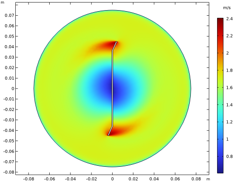
In the Settings window for 2D Plot Group, type Number of Particles and Velocity in the Label text field.
3
Locate the Data section. From the Parameter value (W) list, choose 1.
4
From the Time (s) list, choose 5.
5
Click to expand the Title section. From the Title type list, choose None.
6
Locate the Plot Settings section. From the Frame list, choose Spatial  (x, y, z).
7
Locate the Color Legend section. Select the Show maximum and minimum values checkbox.
8
Select the Show units checkbox.
Surface 1
1
In the Model Builder window, expand the Number of Particles and Velocity node, then click Surface 1.
2
In the Settings window for Surface, locate the Expression section.
3
In the Expression text field, type pbsb.N.
Number of Particles and Velocity
In the Number of Particles and Velocity toolbar, click  Surface.
Surface 2
1
In the Settings window for Surface, locate the Coloring and Style section.
2
From the Color table list, choose RanaArvalis.
Filter 1
1
In the Number of Particles and Velocity toolbar, click  Filter.
2
In the Settings window for Filter, locate the Element Selection section.
3
In the Logical expression for inclusion text field, type x-y>0.
Number of Particles and Velocity
In the Number of Particles and Velocity toolbar, click  Annotation.
Annotation 1
1
In the Settings window for Annotation, locate the Annotation section.
2
In the Text text field, type Particle\\concentration.
3
Select the LaTeX markup checkbox.
4
Locate the Position section. In the x text field, type -0.04.
5
In the y text field, type 0.07.
6
Locate the Coloring and Style section. Clear the Show point checkbox.
7
From the Anchor point list, choose Middle right.
Number of Particles and Velocity
In the Number of Particles and Velocity toolbar, click  Annotation.
Annotation 2
1
In the Settings window for Annotation, locate the Annotation section.
2
In the Text text field, type Velocity.
3
Locate the Position section. In the x text field, type 0.05.
4
In the y text field, type -0.06.
5
Locate the Coloring and Style section. Clear the Show point checkbox.
6
From the Anchor point list, choose Middle left.
7
In the Number of Particles and Velocity toolbar, click  Plot.
Velocity (spf)
1
In the Model Builder window, under Results click Velocity (spf).
2
In the Settings window for 2D Plot Group, locate the Title section.
3
From the Title type list, choose None.
4
Locate the Color Legend section. Select the Show units checkbox.
Pressure (spf), Velocity (spf), Wall Resolution (spf)
1
In the Model Builder window, under Results, Ctrl-click to select Velocity (spf), Pressure (spf), and Wall Resolution (spf).
2
Fluid Flow
In the Settings window for Group, type Fluid Flow in the Label text field.
Number of Particles at Different Times
1
In the Model Builder window, under Results click Population Number Density, n1 (pbsb).
2
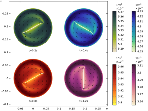
In the Settings window for 2D Plot Group, type Number of Particles at Different Times in the Label text field.
3
Locate the Title section. From the Title type list, choose None.
4
Locate the Plot Settings section. Clear the Plot dataset edges checkbox.
5
Locate the Color Legend section. Select the Show units checkbox.
6
From the Position list, choose Right double.
7
Click to expand the Plot Array section. From the Array type list, choose Square.
Surface 1
1
In the Model Builder window, expand the Number of Particles at Different Times node, then click Surface 1.
2
In the Settings window for Surface, locate the Data section.
3
From the Dataset list, choose Population balance/Solution 1 (sol1).
4
From the Parameter value (W) list, choose 1.
5
From the Time (s) list, choose 0.2.
6
Locate the Expression section. In the Expression text field, type pbsb.N.
7
Locate the Coloring and Style section. From the Color table list, choose Algae.
8
Click to expand the Plot Array section. Select the Manual indexing checkbox.
9
In the Row index text field, type 1.
Arrow Surface 1
1
In the Model Builder window, click Arrow Surface 1.
2
In the Settings window for Arrow Surface, locate the Data section.
3
From the Dataset list, choose Population balance/Solution 1 (sol1).
4
From the Time (s) list, choose 0.2.
5
Click to expand the Plot Array section. Select the Manual indexing checkbox.
6
In the Row index text field, type 1.
Number of Particles at Different Times
In the Number of Particles at Different Times toolbar, click  Annotation.
Annotation 1
1
In the Settings window for Annotation, locate the Annotation section.
2
In the Text text field, type t=0.2s.
3
Locate the Position section. In the y text field, type -0.08.
4
Locate the Coloring and Style section. Clear the Show point checkbox.
5
From the Anchor point list, choose Upper middle.
6
Click to expand the Plot Array section. Select the Manual indexing checkbox.
7
In the Row index text field, type 1.
Annotation 1, Arrow Surface 1, Surface 1
1
In the Model Builder window, under Results > Number of Particles at Different Times, Ctrl-click to select Surface 1, Arrow Surface 1, and Annotation 1.
2
Surface 2
1
In the Settings window for Surface, locate the Data section.
2
From the Time (s) list, choose 0.4.
3
Locate the Coloring and Style section. From the Color table list, choose Cynanthus.
4
Locate the Plot Array section. In the Column index text field, type 1.
Arrow Surface 2
1
In the Model Builder window, click Arrow Surface 2.
2
In the Settings window for Arrow Surface, locate the Data section.
3
From the Time (s) list, choose 0.4.
4
Click to expand the Inherit Style section. From the Plot list, choose Arrow Surface 1.
5
Locate the Plot Array section. In the Column index text field, type 1.
Annotation 2
1
In the Model Builder window, click Annotation 2.
2
In the Settings window for Annotation, locate the Annotation section.
3
In the Text text field, type t=0.4s.
4
Locate the Plot Array section. In the Column index text field, type 1.
Annotation 2, Arrow Surface 2, Surface 2
1
In the Model Builder window, under Results > Number of Particles at Different Times, Ctrl-click to select Surface 2, Arrow Surface 2, and Annotation 2.
2
Surface 3
1
In the Settings window for Surface, locate the Data section.
2
From the Time (s) list, choose 0.8.
3
Locate the Coloring and Style section. From the Color table list, choose RanaDraytonii.
4
Locate the Plot Array section. In the Row index text field, type 0.
5
In the Column index text field, type 0.
Arrow Surface 3
1
In the Model Builder window, click Arrow Surface 3.
2
In the Settings window for Arrow Surface, locate the Data section.
3
From the Time (s) list, choose 0.8.
4
Locate the Plot Array section. In the Row index text field, type 0.
5
In the Column index text field, type 0.
Annotation 3
1
In the Model Builder window, click Annotation 3.
2
In the Settings window for Annotation, locate the Annotation section.
3
In the Text text field, type t=0.8s.
4
Locate the Plot Array section. In the Row index text field, type 0.
5
In the Column index text field, type 0.
Annotation 3, Arrow Surface 3, Surface 3
1
In the Model Builder window, under Results > Number of Particles at Different Times, Ctrl-click to select Surface 3, Arrow Surface 3, and Annotation 3.
2
Annotation 4, Arrow Surface 4, Surface 4
1
In the Settings window for Surface, locate the Data section.
2
From the Time (s) list, choose 1.2.
3
Locate the Coloring and Style section. From the Color table list, choose Arctium.
4
Locate the Plot Array section. In the Column index text field, type 1.
Arrow Surface 4
1
In the Model Builder window, click Arrow Surface 4.
2
In the Settings window for Arrow Surface, locate the Data section.
3
From the Time (s) list, choose 1.2.
4
Locate the Plot Array section. In the Column index text field, type 1.
Annotation 4
1
In the Model Builder window, click Annotation 4.
2
In the Settings window for Annotation, locate the Annotation section.
3
In the Text text field, type t=1.2s.
4
Locate the Plot Array section. In the Column index text field, type 1.
Annotation 3, Arrow Surface 3, Surface 3
In the Model Builder window, under Results > Number of Particles at Different Times, Ctrl-click to select Surface 3, Arrow Surface 3, and Annotation 3.
Surface 3
1
Drag and drop below Annotation 1.
2
In the Number of Particles at Different Times toolbar, click  Plot.
Particle Concentrations of Different Sizes
1
In the Model Builder window, under Results click Population Number Density, n7 (pbsb).
2
In the Settings window for 2D Plot Group, type Particle Concentrations of Different Sizes in the Label text field.
3
Locate the Data section. From the Parameter value (W) list, choose 1.
4
Locate the Title section. From the Title type list, choose None.
5
Locate the Plot Settings section. From the Frame list, choose Spatial  (x, y, z).
6
Locate the Color Legend section. Select the Show units checkbox.
7
From the Position list, choose Right double.
8
Locate the Plot Array section. From the Array type list, choose Square.
Surface 1
1
In the Model Builder window, expand the Particle Concentrations of Different Sizes node, then click Surface 1.
2
In the Settings window for Surface, locate the Expression section.
3
In the Expression text field, type n2*pbsb.dL_n2.
4
Locate the Coloring and Style section. From the Color table list, choose Algae.
5
Locate the Plot Array section. Select the Manual indexing checkbox.
6
In the Row index text field, type 1.
Arrow Surface 1
In the Model Builder window, right-click Arrow Surface 1 and choose Delete.
Particle Concentrations of Different Sizes
In the Particle Concentrations of Different Sizes toolbar, click  Annotation.
Annotation 1
1
In the Settings window for Annotation, locate the Annotation section.
2
In the Text text field, type 138-159 nm.
3
Locate the Position section. In the y text field, type -0.08.
4
Locate the Coloring and Style section. Clear the Show point checkbox.
5
From the Anchor point list, choose Upper middle.
6
Locate the Plot Array section. Select the Manual indexing checkbox.
7
In the Row index text field, type 1.
Annotation 1, Surface 1
1
In the Model Builder window, under Results > Particle Concentrations of Different Sizes, Ctrl-click to select Surface 1 and Annotation 1.
2
Surface 2
1
In the Settings window for Surface, locate the Expression section.
2
In the Expression text field, type n4*pbsb.dL_n4.
3
Locate the Coloring and Style section. From the Color table list, choose Cynanthus.
4
Locate the Plot Array section. In the Column index text field, type 1.
Annotation 2
1
In the Model Builder window, click Annotation 2.
2
In the Settings window for Annotation, locate the Annotation section.
3
In the Text text field, type 183-211 nm.
4
Locate the Plot Array section. In the Column index text field, type 1.
Annotation 2, Surface 2
1
In the Model Builder window, under Results > Particle Concentrations of Different Sizes, Ctrl-click to select Surface 2 and Annotation 2.
2
Surface 3
1
In the Settings window for Surface, locate the Expression section.
2
In the Expression text field, type n8*pbsb.dL_n8.
3
Locate the Coloring and Style section. From the Color table list, choose RanaDraytonii.
4
Locate the Plot Array section. In the Row index text field, type 0.
5
In the Column index text field, type 0.
Annotation 3
1
In the Model Builder window, click Annotation 3.
2
In the Settings window for Annotation, locate the Annotation section.
3
In the Text text field, type 321-370 nm.
4
Locate the Plot Array section. In the Row index text field, type 0.
5
In the Column index text field, type 0.
Annotation 3, Surface 3
1
In the Model Builder window, under Results > Particle Concentrations of Different Sizes, Ctrl-click to select Surface 3 and Annotation 3.
2
Surface 4
1
In the Settings window for Surface, locate the Expression section.
2
In the Expression text field, type n12*pbsb.dL_n12.
3
Locate the Coloring and Style section. From the Color table list, choose Arctium.
4
Locate the Plot Array section. In the Column index text field, type 1.
Annotation 4
1
In the Model Builder window, click Annotation 4.
2
In the Settings window for Annotation, locate the Annotation section.
3
In the Text text field, type 564-649 nm.
4
Locate the Plot Array section. In the Column index text field, type 1.
Annotation 3, Surface 3
In the Model Builder window, under Results > Particle Concentrations of Different Sizes, Ctrl-click to select Surface 3 and Annotation 3.
Surface 3
1
Drag and drop below Annotation 1.
2
In the Particle Concentrations of Different Sizes toolbar, click  Plot.
Population Number Density, n13 (pbsb)
In the Model Builder window, under Results right-click Population Number Density, n13 (pbsb) and choose Delete.
Line Segments 1
1
In the Model Builder window, expand the Average Size Distribution (pbsb) node, then click Line Segments 1.
2
In the Settings window for Line Segments, locate the Data section.
3
From the Dataset list, choose Average 1.
4
From the Parameter selection (W) list, choose First.
5
From the Time selection list, choose First.
6
Click to expand the Coloring and Style section. From the Color list, choose Black.
7
From the Width list, choose 2.
8
Click to expand the Legends section. Select the Show legends checkbox.
9
From the Legends list, choose Manual.
10
Line Segments 2
1
Right-click Results > Average Size Distribution (pbsb) > Line Segments 1 and choose Duplicate.
2
In the Settings window for Line Segments, locate the Data section.
3
From the Parameter selection (W) list, choose All.
4
From the Time selection list, choose From list.
5
In the Times (s) list box, select 3.
6
Locate the Coloring and Style section. Find the Line style subsection. From the Line list, choose Dotted.
7
From the Color list, choose Cycle (reset).
8
Locate the Legends section. From the Legends list, choose Automatic.
Line Segments 3
1
Right-click Line Segments 2 and choose Duplicate.
2
In the Settings window for Line Segments, locate the Data section.
3
In the Times (s) list box, select 6.
4
Locate the Coloring and Style section. Find the Line style subsection. From the Line list, choose Dashed.
Line Segments 4
1
Right-click Line Segments 3 and choose Duplicate.
2
In the Settings window for Line Segments, locate the Data section.
3
From the Time selection list, choose Last.
4
Locate the Coloring and Style section. Find the Line style subsection. From the Line list, choose Dash-dot.
5
In the Average Size Distribution (pbsb) toolbar, click  Plot.
6
Click the  x-Axis Log Scale button in the Graphics toolbar.
Average Size and Number of Particles
1
In the Results toolbar, click  1D Plot Group.
2
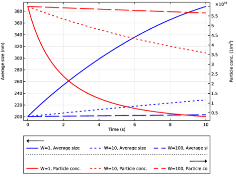
In the Settings window for 1D Plot Group, type Average Size and Number of Particles in the Label text field.
3
Locate the Data section. From the Dataset list, choose Average 1.
4
Click to expand the Title section. From the Title type list, choose None.
5
Locate the Plot Settings section. Select the Two y-axes checkbox.
6
Locate the Legend section. From the Layout list, choose Outside graph axis area.
7
From the Position list, choose Bottom.
Global 1
1
In the Average Size and Number of Particles toolbar, click  Global.
2
In the Settings window for Global, locate the y-Axis Data section.
3
4
Click to expand the Coloring and Style section. Find the Line style subsection. From the Line list, choose Cycle (reset).
5
From the Color list, choose Blue.
6
From the Width list, choose 2.
Average Size and Number of Particles
In the Average Size and Number of Particles toolbar, click  Global.
Global 2
1
In the Settings window for Global, locate the y-Axis Data section.
2
3
Locate the y-Axis section. Select the Plot on secondary y-axis checkbox.
4
Locate the Coloring and Style section. Find the Line style subsection. From the Line list, choose Cycle (reset).
5
From the Color list, choose Red.
6
From the Width list, choose 2.
7
In the Average Size and Number of Particles toolbar, click  Plot.
Volume Conservation
1
In the Results toolbar, click  Evaluation Group.
2
In the Settings window for Evaluation Group, type Volume Conservation in the Label text field.
3
Locate the Transformation section. From the Transformation type list, choose General.
4
Select the Keep child nodes checkbox.
5
In the Expression text field, type abs(int1-int2)/int1.
6
In the Column header text field, type Relative volume change.
7
Click to expand the Format section. From the Include parameters list, choose Off.
Surface Integration 1
1
In the Volume Conservation toolbar, click  Integration and choose Surface Integration.
2
In the Settings window for Surface Integration, locate the Data section.
3
From the Dataset list, choose Population balance/Solution 1 (sol1).
4
From the Time selection list, choose First.
5
6
Locate the Expressions section. In the table, enter the following settings:
Volume Conservation
In the Volume Conservation toolbar, click  Integration and choose Surface Integration.
Surface Integration 2
1
In the Settings window for Surface Integration, locate the Data section.
2
From the Dataset list, choose Population balance/Solution 1 (sol1).
3
From the Time selection list, choose Last.
4
5
Locate the Expressions section. In the table, enter the following settings:
6
In the Volume Conservation toolbar, click  Evaluate.