|
|
|

|
1
|
|
2
|
|
3
|
Click Add.
|
|
4
|
Click
|
|
5
|
|
6
|
Click
|
|
1
|
|
2
|
|
3
|
Click
|
|
4
|
Browse to the model’s Application Libraries folder and double-click the file tortuous_reactor_parameters.txt.
|
|
1
|
|
2
|
|
3
|
|
4
|
|
1
|
|
2
|
|
3
|
|
4
|
|
5
|
|
6
|
Locate the Reaction Orders section. Find the Surface overall reaction order subsection. In the Forward text field, type 0.
|
|
7
|
|
8
|
|
9
|
|
1
|
|
2
|
|
3
|
|
4
|
|
5
|
Locate the Reaction Orders section. Find the Surface overall reaction order subsection. In the Forward text field, type 0.
|
|
6
|
|
7
|
|
8
|
|
9
|
|
1
|
|
2
|
|
3
|
Select the Keep concentration/activity constant checkbox.
|
|
4
|
|
5
|
|
6
|
|
7
|
|
1
|
|
2
|
|
4
|
Locate the Surface Species Initial Values section. In the table, enter the following settings:
|
|
1
|
|
2
|
|
3
|
Select the Auxiliary sweep checkbox.
|
|
4
|
Click
|
|
6
|
|
1
|
|
2
|
|
3
|
|
4
|
|
5
|
|
6
|
|
7
|
|
8
|
|
9
|
|
10
|
|
11
|
|
12
|
|
13
|
|
1
|
|
2
|
|
3
|
|
4
|
|
1
|
|
2
|
|
3
|
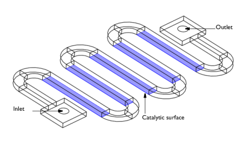
Browse to the model’s Application Libraries folder and double-click the file tortuous_reactor_geom_sequence.mph.
|
|
4
|
|
5
|
|
1
|
|
2
|
Go to the Add Material window.
|
|
3
|
|
4
|
Click the Add to Component button in the window toolbar.
|
|
5
|
|
1
|
|
2
|
|
3
|
|
1
|
|
2
|
|
3
|
|
1
|
|
2
|
|
3
|
|
1
|
|
2
|
|
3
|
|
1
|
In the Model Builder window, expand the Transport of Diluted Species (tds) node, then click Fluid 1.
|
|
2
|
|
3
|
|
4
|
|
5
|
|
1
|
|
2
|
|
3
|
|
1
|
|
2
|
|
3
|
|
4
|
|
5
|
|
6
|
Select the Species cRH checkbox.
|
|
7
|
|
8
|
Select the Species cRR checkbox.
|
|
9
|
|
1
|
|
2
|
|
3
|
|
1
|
In the Model Builder window, expand the Component 2 (comp2) > Laminar Flow (spf) node, then click Fluid Properties 1.
|
|
2
|
|
3
|
|
1
|
|
2
|
|
3
|
|
4
|
|
5
|
|
1
|
|
2
|
|
3
|
|
1
|
|
2
|
|
3
|
Click
|
|
4
|
|
5
|
Click OK.
|
|
1
|
|
2
|
|
3
|
Click the Custom button.
|
|
4
|
Locate the Element Size Parameters section.
|
|
5
|
|
1
|
|
2
|
|
3
|
|
4
|
|
1
|
|
2
|
|
3
|
|
1
|
|
2
|
|
3
|
|
4
|
|
1
|
|
2
|
|
3
|
Click the Custom button.
|
|
4
|
Locate the Element Size Parameters section.
|
|
5
|
|
6
|
|
1
|
|
2
|
|
3
|
In the Solve for column of the table, under Component 2 (comp2), clear the checkbox for Transport of Diluted Species (tds).
|
|
4
|
|
5
|
Click
|
|
1
|
|
2
|
|
3
|
In the Solve for column of the table, under Component 2 (comp2), clear the checkbox for Laminar Flow (spf).
|
|
4
|
|
5
|
Click
|
|
7
|
Click to expand the Values of Dependent Variables section. Find the Values of variables not solved for subsection. From the Settings list, choose User controlled.
|
|
8
|
|
9
|
|
10
|
|
11
|
|
1
|
|
2
|
|
3
|
|
4
|
|
1
|
In the Model Builder window, expand the Concentration, RBr, Surface (tds) node, then click Surface 1.
|
|
2
|
|
3
|
|
1
|
|
2
|
|
3
|
|
4
|
|
1
|
|
2
|
|
3
|
Select the Show units checkbox.
|
|
1
|
|
2
|
|
3
|
|
4
|
|
5
|
|
1
|
|
2
|
|
3
|
|
4
|
Click
|
|
5
|
|
6
|
Click OK.
|
|
7
|
|
8
|
|
9
|
Click
|
|
10
|
Click
|
|
11
|
|
12
|
Click OK.
|
|
1
|
|
2
|
|
3
|
|
4
|
Click
|
|
5
|
|
6
|
Click OK.
|
|
1
|
|
2
|
|
3
|
|
4
|
Click
|
|
5
|
|
6
|
Click OK.
|
|
1
|
|
2
|
|
3
|
|
4
|
Click
|
|
5
|
|
6
|
Click OK.
|
|
1
|
|
2
|
|
3
|
|
4
|
Click
|
|
5
|
|
6
|
Click OK.
|
|
1
|
|
2
|
|
3
|
|
4
|
Click
|
|
5
|
|
6
|
Click OK.
|
|
1
|
|
2
|
|
1
|
|
2
|
|
1
|
|
2
|
|
1
|
|
2
|
|
3
|
|
4
|
|
5
|
|
6
|
Click
|
|
7
|
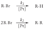
Browse to the model’s Application Libraries folder and double-click the file tortuous_reactor_RBr_evaluation_group_expressions.txt.
|
|
1
|
|
2
|
|
3
|
Select the Transpose checkbox.
|
|
4
|
|
5
|
|
1
|
|
2
|
|
3
|
|
4
|
|
5
|
|
6
|
Click
|
|
7
|
Browse to the model’s Application Libraries folder and double-click the file tortuous_reactor_RH_evaluation_group_expressions.txt.
|
|
1
|
|
2
|
|
3
|
Select the Transpose checkbox.
|
|
4
|
|
5
|
|
1
|
|
2
|
|
3
|
|
4
|
|
5
|
|
6
|
Click
|
|
7
|
Browse to the model’s Application Libraries folder and double-click the file tortuous_reactor_RR_evaluation_group_expressions.txt.
|
|
1
|
|
2
|
|
3
|
Select the Transpose checkbox.
|
|
4
|
|
5
|
|
1
|
|
2
|
|
3
|
|
4
|
Click
|
|
5
|
|
6
|
Click OK.
|
|
1
|
|
2
|
|
3
|
|
4
|
|
5
|
Locate the Plot Settings section.
|
|
6
|
|
7
|
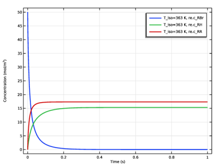
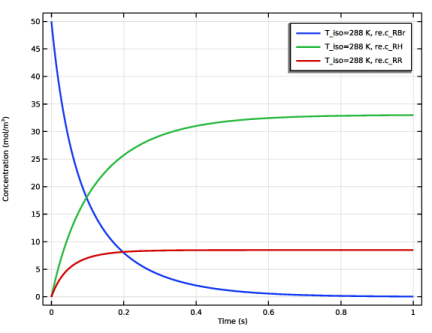
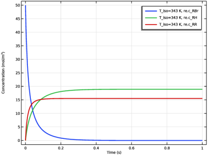
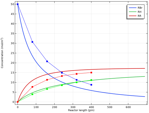
Select the y-axis label checkbox. In the associated text field, type Concentration (mol/m<sup>3</sup>).
|
|
1
|
|
2
|
|
3
|
|
4
|
|
5
|
|
6
|
|
7
|
|
8
|
|
9
|
|
10
|
|
12
|
|
1
|
|
2
|
|
3
|
|
4
|
|
5
|
Click to expand the Preprocessing section. Find the x-axis column subsection. From the Transformation list, choose Linear.
|
|
6
|
|
7
|
|
8
|
|
9
|
|
1
|
|
2
|
|
3
|
|
4
|
|
1
|
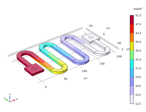
In the Model Builder window, expand the Results > 0D versus 3D concentrations > Table Graph 2 node, then click Results > 0D versus 3D concentrations > Table Graph 3.
|
|
2
|
|
3
|
|
4
|
|
1
|
|
2
|
|
3
|
|
1
|
|
2
|
|
1
|
|
2
|
|
3
|
|
4
|
|
5
|
|
6
|
|
7
|
|
8
|
Locate the Selections of Resulting Entities section. Find the Cumulative selection subsection. Click New.
|
|
9
|
|
10
|
Click OK.
|
|
1
|
|
2
|
|
3
|
|
4
|
Locate the Selections of Resulting Entities section. Find the Cumulative selection subsection. From the Contribute to list, choose Channel.
|
|
5
|
|
6
|
|
1
|
|
2
|
|
3
|
|
4
|
|
5
|
|
6
|
|
7
|
Click to expand the Layers section. In the table, enter the following settings:
|
|
8
|
Locate the Selections of Resulting Entities section. Find the Cumulative selection subsection. From the Contribute to list, choose Channel.
|
|
1
|
|
2
|
|
3
|
|
4
|
|
1
|
|
2
|
|
3
|
|
4
|
|
5
|
|
6
|
|
1
|
|
2
|
|
3
|
|
4
|
|
5
|
|
6
|
|
7
|
|
8
|
Locate the Selections of Resulting Entities section. Find the Cumulative selection subsection. Click New.
|
|
9
|
|
10
|
Click OK.
|
|
1
|
|
2
|
|
3
|
|
4
|
|
1
|
|
2
|
|
3
|
|
4
|
|
5
|
|
1
|
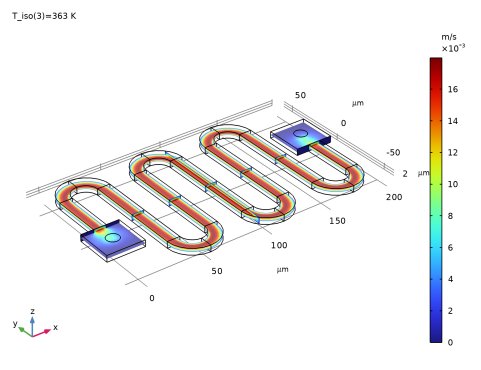
In the Model Builder window, under Component 1 (comp1) > Geometry 1 right-click Work Plane 1 (wp1) and choose Transforms > Rotate.
|
|
2
|
|
3
|
|
4
|
Select the Keep input objects checkbox.
|
|
5
|
|
6
|
|
7
|
Locate the Selections of Resulting Entities section. Find the Cumulative selection subsection. From the Contribute to list, choose Adapter Sections.
|
|
1
|
|
2
|
|
3
|
|
4
|
|
5
|
|
6
|
Locate the Selections of Resulting Entities section. Find the Cumulative selection subsection. From the Contribute to list, choose Channel.
|
|
1
|
|
2
|
|
3
|
|
4
|
|
5
|
Click
|
|
6
|
|
1
|
|
2
|
|
3
|
|
4
|
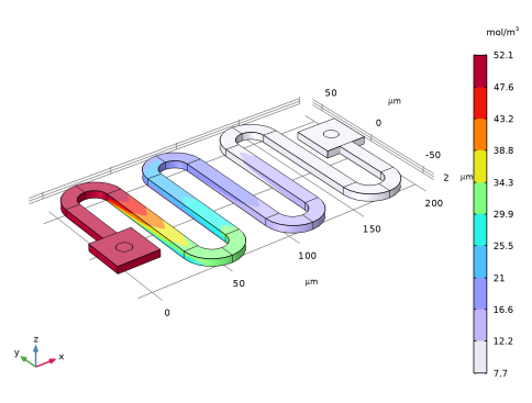
On the object arr2(1,1,1,1), select Domains 2, 3, and 5 only.
|
|
5
|
On the object arr2(1,1,1,2), select Domains 1, 3, and 4 only.
|
|
6
|
On the object arr2(2,1,1,1), select Domains 2, 3, and 5 only.
|
|
7
|
On the object arr2(2,1,1,2), select Domains 1, 3, and 4 only.
|
|
8
|
On the object arr2(3,1,1,1), select Domains 2, 3, and 5 only.
|
|
9
|
On the object arr2(3,1,1,2), select Domains 1, 3, and 4 only.
|
|
1
|
|
2
|
|
1
|
|
2
|
|
3
|
|
4
|
On the object fin, select Boundary 6 only.
|
|
1
|
|
2
|
|
3
|
|
4
|
On the object fin, select Boundary 109 only.
|
|
1
|
|
2
|
|
3
|
|
4
|
|
5
|
Click
|
|
6
|
|
7
|
Click OK.
|
|
8
|
|
9
|
|
10
|
|
11
|
|
12
|
|
13
|
|
14
|
|
15
|
|
1
|
|
2
|
|
3
|
Click
|
|
4
|
|
5
|
Click OK.
|
|
6
|
In the Settings window for Adjacent Selection, type Adjacent Selection - Walls in the Label text field.
|
|
1
|
|
2
|
|
3
|
|
4
|
|
5
|
|
6
|
Click OK.
|
|
7
|
|
8
|
|
9
|
|
10
|
Click OK.
|