
|
|
|

|
1
|
|
2
|
In the Select Physics tree, select Chemical Species Transport > Transport of Concentrated Species (tcs).
|
|
3
|
Click Add.
|
|
4
|
|
5
|
In the Mass fractions (1) table, enter the following settings:
|
|
6
|
|
7
|
Click Add.
|
|
8
|
Click
|
|
9
|
|
10
|
Click
|
|
1
|
|
2
|
|
3
|
Click
|
|
4
|
Browse to the model’s Application Libraries folder and double-click the file thin_domain_parameters.txt.
|
|
1
|
|
2
|
|
3
|
|
4
|
|
5
|
Click
|
|
1
|
In the Model Builder window, under Component 1 (comp1) click Transport of Concentrated Species (tcs).
|
|
2
|
In the Settings window for Transport of Concentrated Species, locate the Out-of-Plane Thickness section.
|
|
3
|
|
4
|
|
1
|
In the Model Builder window, under Component 1 (comp1) > Transport of Concentrated Species (tcs) click Species Molar Masses 1.
|
|
2
|
|
3
|
|
4
|
|
5
|
|
1
|
|
1
|
|
2
|
|
3
|
|
4
|
|
1
|
|
1
|
|
2
|
|
3
|
Select the Species wA_2D checkbox.
|
|
4
|
|
1
|
|
2
|
|
3
|
|
4
|
Select the Use shallow channel approximation checkbox.
|
|
5
|
|
1
|
In the Model Builder window, under Component 1 (comp1) > Laminar Flow (spf) click Fluid Properties 1.
|
|
2
|
|
3
|
|
1
|
|
1
|
|
3
|
|
4
|
From the list, choose Fully developed flow.
|
|
5
|
|
1
|
|
1
|
|
2
|
|
3
|
From the list, choose User-controlled mesh.
|
|
1
|
In the Model Builder window, under Component 1 (comp1) > Mesh 1, Ctrl-click to select Size 1, Corner Refinement 1, and Free Triangular 1.
|
|
2
|
Right-click and choose Delete.
|
|
1
|
|
2
|
Drag and drop below Size.
|
|
1
|
|
2
|
Select Boundaries 2 and 3 only, the two boundaries parallel to the x-axis, that is, in the direction of the incoming flow.
|
|
3
|
|
4
|
|
5
|
|
6
|
|
7
|
Select the Symmetric distribution checkbox.
|
|
8
|
Click
|
|
1
|
|
3
|
|
4
|
|
5
|
|
6
|
|
7
|
Select the Reverse direction checkbox.
|
|
8
|
Click
|
|
1
|
In the Model Builder window, expand the Component 1 (comp1) > Mesh 1 > Boundary Layers 1 node, then click Boundary Layer Properties 1.
|
|
2
|
|
3
|
|
4
|
|
1
|
|
2
|
|
3
|
Clear the Smooth transition to interior mesh checkbox.
|
|
4
|
Click
|
|
1
|
|
2
|
|
3
|
Click
|
|
5
|
|
1
|
|
2
|
Go to the Result Templates window.
|
|
3
|
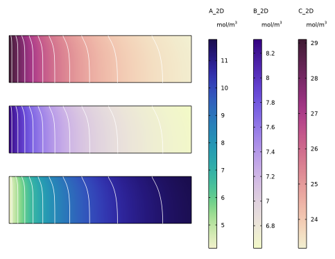
In the tree, select Study 1/Solution 1 (sol1) > Transport of Concentrated Species > Plot array: Concentrations, A_2D, B_2D, C_2D (tcs).
|
|
4
|
Click the Add Result Template button in the window toolbar.
|
|
5
|
|
1
|
|
2
|
|
3
|
|
4
|
|
1
|
In the Model Builder window, under Results > Plot array: Concentrations, A_2D, B_2D, C_2D (tcs), Ctrl-click to select Total Flux, A_2D, Total Flux, B_2D, and Total Flux, C_2D.
|
|
2
|
Right-click and choose Delete.
|
|
1
|
|
2
|
|
3
|
|
4
|
|
5
|
|
6
|
Clear the Color legend checkbox.
|
|
7
|
|
1
|
|
2
|
|
3
|
|
4
|
|
5
|
|
6
|
Clear the Color legend checkbox.
|
|
7
|
|
8
|
|
1
|
|
2
|
|
3
|
|
4
|
|
5
|
|
6
|
Clear the Color legend checkbox.
|
|
7
|
|
8
|
|
1
|
|
2
|
|
3
|
|
4
|
|
5
|
|
6
|
|
1
|
In the Model Builder window, under Results > Plot array: Concentrations, A_2D, B_2D, C_2D (tcs), Ctrl-click to select A_2D, B_2D, and C_2D.
|
|
2
|
|
1
|
|
2
|
|
3
|
|
4
|
|
5
|
|
1
|
|
2
|
|
4
|
|
5
|
|
6
|
|
7
|
Click to expand the Coloring and Style section. Find the Line style subsection. From the Line list, choose Dashed.
|
|
8
|
|
9
|
|
10
|
|
1
|
|
3
|
|
4
|
|
5
|
|
6
|
Locate the Coloring and Style section. Find the Line style subsection. From the Line list, choose Dashed.
|
|
7
|
|
8
|
|
9
|
|
1
|
|
3
|
|
4
|
|
5
|
|
6
|
Locate the Coloring and Style section. Find the Line style subsection. From the Line list, choose Dashed.
|
|
7
|
|
8
|
|
9
|
|
10
|
|
1
|
|
2
|
Go to the Result Templates window.
|
|
3
|
In the tree, select Study 1/Solution 1 (sol1) > Transport of Concentrated Species > Mass Balance, A_2D (tcs) and Study 1/Solution 1 (sol1) > Transport of Concentrated Species > Mass Balance, B_2D (tcs).
|
|
4
|
Click the Add Result Template button in the window toolbar.
|
|
5
|
|
1
|
|
2
|
|
3
|
|
4
|
|
1
|
|
2
|
|
3
|
|
4
|
|
5
|
|
1
|
|
2
|
|
3
|
|
4
|
|
5
|
|
6
|
Click
|
|
1
|
|
2
|
|
1
|
|
2
|
Go to the Add Physics window.
|
|
3
|
|
4
|
Find the Physics interfaces in study subsection. In the table, clear the Solve checkbox for Study 1.
|
|
5
|
Click the Add to Component 2 button in the window toolbar.
|
|
6
|
|
7
|
|
8
|
Click the Add to Component 2 button in the window toolbar.
|
|
9
|
|
1
|
In the Settings window for Transport of Concentrated Species, click to expand the Dependent Variables section.
|
|
2
|
|
3
|
In the Mass fractions (1) table, enter the following settings:
|
|
4
|
|
1
|
In the Model Builder window, under Component 2 (comp2) > Transport of Concentrated Species 2 (tcs2) click Species Molar Masses 1.
|
|
2
|
|
3
|
|
4
|
|
5
|
|
1
|
|
1
|
|
2
|
|
3
|
|
4
|
|
1
|
|
1
|
|
3
|
|
4
|
Select the Account for Stefan velocity checkbox.
|
|
5
|
|
6
|
|
1
|
|
2
|
|
3
|
|
1
|
In the Model Builder window, under Component 2 (comp2) > Laminar Flow 2 (spf2) click Fluid Properties 1.
|
|
2
|
|
3
|
|
1
|
|
1
|
|
2
|
|
3
|
From the list, choose Fully developed flow.
|
|
4
|
|
1
|
|
2
|
|
3
|
Select the Normal flow checkbox.
|
|
1
|
|
2
|
Go to the Add Physics window.
|
|
3
|
|
1
|
|
2
|
|
3
|
From the list, choose User-controlled mesh.
|
|
1
|
In the Model Builder window, under Component 2 (comp2) > Mesh 2, Ctrl-click to select Size 1, Size 2, Corner Refinement 1, and Free Tetrahedral 1.
|
|
2
|
Right-click and choose Delete.
|
|
1
|
|
2
|
Drag and drop below Size.
|
|
1
|
|
3
|
|
4
|
|
5
|
|
6
|
|
7
|
Select the Symmetric distribution checkbox.
|
|
8
|
Click
|
|
1
|
|
1
|
In the Model Builder window, under Component 2 (comp2) > Mesh 2 > Mapped 1 right-click Distribution 1 and choose Duplicate.
|
|
3
|
|
4
|
|
5
|
|
6
|
Clear the Symmetric distribution checkbox.
|
|
7
|
Click
|
|
1
|
|
2
|
|
3
|
|
4
|
|
5
|
|
6
|
Select the Symmetric distribution checkbox.
|
|
1
|
|
2
|
|
3
|
|
1
|
In the Model Builder window, expand the Boundary Layers 1 node, then click Boundary Layer Properties 1.
|
|
2
|
In the Settings window for Boundary Layer Properties, locate the Geometric Entity Selection section.
|
|
3
|
Click
|
|
1
|
|
2
|
|
3
|
Clear the Smooth transition to interior mesh checkbox.
|
|
4
|
Click
|
|
1
|
|
2
|
Go to the Add Study window.
|
|
3
|
Find the Physics interfaces in study subsection. In the table, clear the Solve checkboxes for Transport of Concentrated Species (tcs) and Laminar Flow (spf).
|
|
4
|
Find the Multiphysics couplings in study subsection. In the table, clear the Solve checkbox for Reacting Flow 1 (nirf1).
|
|
5
|
|
6
|
Click the Add Study button in the window toolbar.
|
|
7
|
|
1
|
|
2
|
|
3
|
Click
|
|
5
|
|
1
|
|
2
|
|
3
|
|
4
|
|
1
|
|
2
|
|
3
|
|
1
|
|
2
|
|
3
|
|
4
|
|
1
|
|
2
|
|
3
|
|
1
|
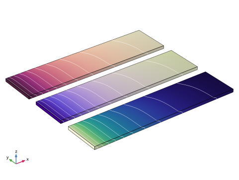
In the Model Builder window, under Results, Ctrl-click to select Concentration, A_3D, Streamline (tcs2), Concentration, A_3D, Surface (tcs2), Concentration, B_3D, Streamline (tcs2), Concentration, B_3D, Surface (tcs2), Concentration, C_3D, Streamline (tcs2), and Concentration, C_3D, Surface (tcs2).
|
|
2
|
Right-click and choose Delete.
|
|
1
|
|
2
|
Go to the Result Templates window.
|
|
3
|
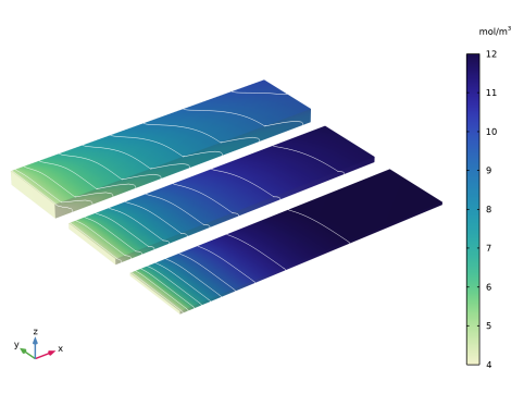
In the tree, select Study 2/Parametric Solutions 1 (5) (sol3) > Transport of Concentrated Species 2 > Plot array: Concentrations, A_3D, B_3D, C_3D (tcs2).
|
|
4
|
Click the Add Result Template button in the window toolbar.
|
|
5
|
|
1
|
|
2
|
|
3
|
|
4
|
|
5
|
|
6
|
|
1
|
|
2
|
|
3
|
|
4
|
|
5
|
|
6
|
|
7
|
Clear the Color legend checkbox.
|
|
8
|
|
9
|
|
1
|
|
2
|
|
3
|
|
4
|
|
5
|
|
6
|
Clear the Color legend checkbox.
|
|
7
|
|
8
|
|
1
|
|
2
|
|
3
|
|
4
|
|
5
|
|
6
|
Clear the Color legend checkbox.
|
|
7
|
|
8
|
|
9
|
|
1
|
|
2
|
|
3
|
|
4
|
|
5
|
|
6
|
|
7
|
|
1
|
|
2
|
|
3
|
|
4
|
|
5
|
|
6
|
|
7
|
|
8
|
|
9
|
|
10
|
|
1
|
|
2
|
|
3
|
|
4
|
|
5
|
|
6
|
|
7
|
|
8
|
Clear the Color legend checkbox.
|
|
9
|
|
1
|
|
2
|
|
3
|
|
4
|
|
5
|
|
6
|
|
7
|
|
8
|
|
9
|
Clear the Color legend checkbox.
|
|
10
|
|
11
|
|
1
|
|
2
|
|
3
|
|
4
|
|
5
|
|
6
|
|
7
|
|
8
|
Clear the Color legend checkbox.
|
|
9
|
|
10
|
|
1
|
|
2
|
|
3
|
|
4
|
|
5
|
|
6
|
|
7
|
|
8
|
Clear the Color legend checkbox.
|
|
9
|
|
10
|
|
1
|
|
2
|
|
3
|
|
4
|
|
5
|
|
6
|
|
7
|
Clear the Color legend checkbox.
|
|
8
|
|
9
|
|
10
|
|
1
|
|
2
|
|
3
|
|
4
|
|
5
|
|
7
|
|
8
|
|
9
|
|
10
|
|
1
|
|
2
|
|
3
|
|
4
|
|
6
|
|
7
|
|
8
|
|
1
|
|
2
|
|
3
|
|
4
|
|
6
|
|
7
|
|
8
|
|
9
|
|
1
|
|
2
|
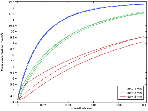
In the Settings window for 1D Plot Group, type Species A Concentration Along Center in the Label text field.
|
|
3
|
|
4
|
|
1
|
|
2
|
|
3
|
|
5
|
|
6
|
|
7
|
|
8
|
Locate the Coloring and Style section. Find the Line style subsection. From the Line list, choose Dashed.
|
|
1
|
|
2
|
|
4
|
|
5
|
|
6
|
|
7
|
|
8
|
|
9
|
|
10
|
|
1
|
|
2
|
|
3
|
|
4
|
|
1
|
|
2
|
Go to the Result Templates window.
|
|
3
|
In the tree, select Study 2/Parametric Solutions 1 (5) (sol3) > Transport of Concentrated Species 2 > Mass Balance, A_3D (tcs2) and Study 2/Parametric Solutions 1 (5) (sol3) > Transport of Concentrated Species 2 > Mass Balance, B_3D (tcs2).
|
|
4
|
Click the Add Result Template button in the window toolbar.
|
|
1
|
|
2
|
|
3
|
|
4
|
|
1
|
|
2
|
|
3
|
|
4
|
|
5
|
 ,
,