|
|
|

|
Normal, σ/E=0.3%
|
|||
|
Normal, σ/A=10%
|
|||
|
Normal, σ/D_BetaC_ref=20%
|
|||
|
-
|
For example, what is P(c < cmin), the probability that the outlet concentration is below some minimum value?
|
|
1
|
|
2
|
In the Select Physics tree, select Chemical Species Transport > Reacting Flow > Laminar Flow, Diluted Species.
|
|
3
|
Click Add.
|
|
4
|
|
5
|
Click
|
|
6
|
In the Concentrations (mol/m³) table, enter the following settings:
|
|
7
|
|
8
|
Click Add.
|
|
9
|
Click
|
|
10
|
|
11
|
Click
|
|
1
|
|
2
|
|
3
|
Click
|
|
4
|
Browse to the model’s Application Libraries folder and double-click the file thermal_decomposition_uq_parameters.txt.
|
|
1
|
|
2
|
|
3
|
|
4
|
|
5
|
|
1
|
|
2
|
|
3
|
|
4
|
|
1
|
|
2
|
|
3
|
|
4
|
|
5
|
|
1
|
|
2
|
On the object c1, select Point 3 only.
|
|
3
|
|
4
|
|
5
|
|
6
|
|
1
|
|
2
|
Select the object r1 only.
|
|
3
|
|
4
|
|
5
|
|
1
|
|
2
|
On the object fin, select Boundary 6 only.
|
|
3
|
|
1
|
|
2
|
|
3
|
|
4
|
|
6
|
|
1
|
|
2
|
|
1
|
|
2
|
|
1
|
|
2
|
|
1
|
|
2
|
|
3
|
|
4
|
|
6
|
|
7
|
|
1
|
In the Model Builder window, expand the Boundary Layers 1 node, then click Boundary Layer Properties 1.
|
|
2
|
|
3
|
|
4
|
|
1
|
Right-click Component 1 (comp1) > Mesh 1 > Boundary Layers 1 > Boundary Layer Properties 1 and choose Duplicate.
|
|
2
|
|
3
|
|
4
|
|
5
|
|
1
|
|
2
|
|
3
|
|
4
|
Click
|
|
1
|
In the Model Builder window, under Component 1 (comp1) right-click Definitions and choose Variables.
|
|
2
|
|
1
|
|
2
|
Go to the Add Material window.
|
|
3
|
|
4
|
Click Search.
|
|
5
|
|
6
|
Click the Add to Component button in the window toolbar.
|
|
7
|
|
1
|
|
1
|
|
1
|
|
1
|
|
1
|
|
2
|
|
3
|
|
1
|
|
3
|
|
4
|
|
1
|
|
2
|
Go to the Add Physics window.
|
|
3
|
|
4
|
Click the Add to Component 1 button in the window toolbar.
|
|
5
|
|
1
|
|
2
|
|
3
|
|
4
|
|
5
|
|
6
|
|
7
|
Locate the Reaction Thermodynamic Properties section. From the Enthalpy of reaction list, choose User defined.
|
|
8
|
|
1
|
|
2
|
|
3
|
|
1
|
|
2
|
|
3
|
|
4
|
|
5
|
|
6
|
Find the Bulk species subsection. From the Species solved for list, choose Transport of Diluted Species.
|
|
1
|
|
3
|
|
4
|
|
5
|
|
1
|
In the Model Builder window, under Component 1 (comp1) > Transport of Diluted Species (tds) click Fluid 1.
|
|
2
|
|
3
|
|
1
|
|
3
|
|
4
|
|
1
|
|
1
|
|
3
|
|
4
|
|
5
|
|
1
|
|
2
|
|
3
|
From the list, choose Fully developed flow.
|
|
4
|
|
1
|
|
2
|
|
3
|
Select the Normal flow checkbox.
|
|
1
|
|
2
|
In the Solve for column of the table, under Component 1 (comp1), select the checkbox for Laminar Flow (spf).
|
|
3
|
In the Solve for column of the table, under Component 1 (comp1), clear the checkboxes for Transport of Diluted Species (tds), Heat Transfer in Fluids (ht), and Chemistry (chem).
|
|
4
|
|
1
|
|
2
|
|
3
|
|
4
|
|
5
|
|
6
|
|
1
|
|
2
|
|
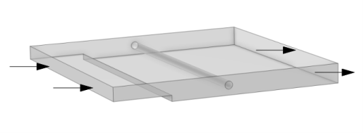
β-carotene outflow
|
|
1
|
|
2
|
|
3
|
Click
|
|
5
|
|
7
|
|
8
|
|
10
|
|
11
|
|
12
|
|
14
|
|
15
|
|
16
|
|
18
|
|
19
|
|
21
|
|
22
|
|
23
|
|
25
|
|
26
|
|
28
|
|
29
|
|
31
|
|
32
|
|
34
|
|
35
|
|
36
|
|
38
|
Locate the Advanced Settings section. From the Error handling list, choose Skip problematic parameters.
|
|
39
|
|
40
|
|
1
|
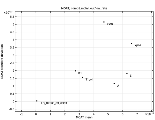
In the Model Builder window, expand the Results > Uncertainty Quantification Graph > MOAT, comp1.molar_outflow_rate node.
|
|
2
|
Right-click Study 2: UQ Screening > Uncertainty Quantification and choose Add New Uncertainty Quantification Study For > Sensitivity Analysis.
|
|
1
|
|
2
|
|
1
|
In the Model Builder window, under Study 3: UQ Sensitivity Analysis click Uncertainty Quantification.
|
|
2
|
|
4
|
Click
|
|
5
|
|
1
|
|
2
|
|
1
|
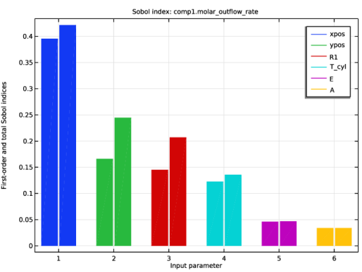
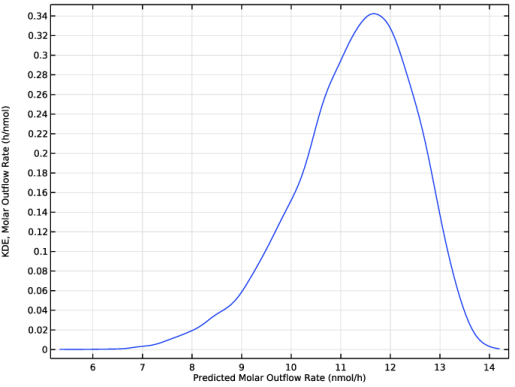
In the Model Builder window, expand the Results > Uncertainty Quantification Graph 2 > Kernel Density Estimation, QoI1 node, then click Line Graph 1.
|
|
2
|
|
3
|
|
4
|
|
5
|
|
6
|
|
1
|
|
2
|
|
3
|
|
4
|
|
1
|
In the Model Builder window, under Study 5: Reliability Analysis, EGRA click Uncertainty Quantification.
|
|
2
|
|
4
|
|
5
|
|
1
|
|
2
|
|
3
|
|
4
|
|
5
|
|
6
|
|
7
|
|
8
|
|
1
|
|
2
|
|
3
|
|
4
|
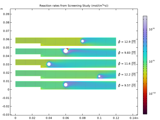
From the Parameter value (T_cyl (K),E (J/mol),A (1/s),H (J/mol),...) list, choose 1: T_cyl=360.15 K, E=1.0898E5 J/mol, A=8.996E13 1/s, H=8652 J/mol, D_BetaC_ref=7.9064E-10 m^2/s, dDdT=3.75E-11 m^2/(s*K), xpos=0.06 m, ypos=0.00575 m, R1=0.002 m.
|
|
5
|
|
6
|
|
7
|
|
8
|
|
9
|
|
1
|
|
2
|
|
3
|
From the Parameter value (T_cyl (K),E (J/mol),A (1/s),H (J/mol),...) list, choose 10: T_cyl=366.82 K, E=1.1014E5 J/mol, A=1.2305E14 1/s, H=8316 J/mol, D_BetaC_ref=2.2479E-9 m^2/s, dDdT=8.75E-11 m^2/(s*K), xpos=0.1 m, ypos=0.00275 m, R1=0.001 m.
|
|
4
|
|
5
|
|
1
|
|
2
|
|
3
|
From the Parameter value (T_cyl (K),E (J/mol),A (1/s),H (J/mol),...) list, choose 20: T_cyl=360.15 K, E=1.1102E5 J/mol, A=9.804E13 1/s, H=8652 J/mol, D_BetaC_ref=7.9064E-10 m^2/s, dDdT=3.75E-11 m^2/(s*K), xpos=0.04 m, ypos=0.00425 m, R1=0.002 m.
|
|
4
|
|
1
|
|
2
|
|
3
|
From the Parameter value (T_cyl (K),E (J/mol),A (1/s),H (J/mol),...) list, choose 30: T_cyl=370.15 K, E=1.0898E5 J/mol, A=8.996E13 1/s, H=8484 J/mol, D_BetaC_ref=3.3494E-9 m^2/s, dDdT=6.25E-11 m^2/(s*K), xpos=0.06 m, ypos=0.00725 m, R1=0.0025 m.
|
|
4
|
|
1
|
|
2
|
|
3
|
From the Parameter value (T_cyl (K),E (J/mol),A (1/s),H (J/mol),...) list, choose 40: T_cyl=363.48 K, E=1.0986E5 J/mol, A=6.4952E13 1/s, H=8148 J/mol, D_BetaC_ref=1.8921E-9 m^2/s, dDdT=1.125E-10 m^2/(s*K), xpos=0.08 m, ypos=0.00575 m, R1=0.0015 m.
|
|
4
|
|
1
|
|
2
|
|
3
|
|
4
|
From the Parameter value (T_cyl (K),E (J/mol),A (1/s),H (J/mol),...) list, choose 1: T_cyl=360.15 K, E=1.0898E5 J/mol, A=8.996E13 1/s, H=8652 J/mol, D_BetaC_ref=7.9064E-10 m^2/s, dDdT=3.75E-11 m^2/(s*K), xpos=0.06 m, ypos=0.00575 m, R1=0.002 m.
|
|
5
|
|
6
|
|
7
|
|
8
|
Locate the Coloring and Style section. Find the Point style subsection. From the Color list, choose Custom.
|
|
9
|
|
10
|
Click Define custom colors.
|
|
12
|
Click Add to custom colors.
|
|
13
|
|
14
|
|
15
|
|
1
|
|
2
|
|
3
|
From the Parameter value (T_cyl (K),E (J/mol),A (1/s),H (J/mol),...) list, choose 10: T_cyl=366.82 K, E=1.1014E5 J/mol, A=1.2305E14 1/s, H=8316 J/mol, D_BetaC_ref=2.2479E-9 m^2/s, dDdT=8.75E-11 m^2/(s*K), xpos=0.1 m, ypos=0.00275 m, R1=0.001 m.
|
|
4
|
|
1
|
|
2
|
|
3
|
From the Parameter value (T_cyl (K),E (J/mol),A (1/s),H (J/mol),...) list, choose 20: T_cyl=360.15 K, E=1.1102E5 J/mol, A=9.804E13 1/s, H=8652 J/mol, D_BetaC_ref=7.9064E-10 m^2/s, dDdT=3.75E-11 m^2/(s*K), xpos=0.04 m, ypos=0.00425 m, R1=0.002 m.
|
|
4
|
|
1
|
|
2
|
|
3
|
From the Parameter value (T_cyl (K),E (J/mol),A (1/s),H (J/mol),...) list, choose 30: T_cyl=370.15 K, E=1.0898E5 J/mol, A=8.996E13 1/s, H=8484 J/mol, D_BetaC_ref=3.3494E-9 m^2/s, dDdT=6.25E-11 m^2/(s*K), xpos=0.06 m, ypos=0.00725 m, R1=0.0025 m.
|
|
4
|
|
1
|
|
2
|
|
3
|
From the Parameter value (T_cyl (K),E (J/mol),A (1/s),H (J/mol),...) list, choose 40: T_cyl=363.48 K, E=1.0986E5 J/mol, A=6.4952E13 1/s, H=8148 J/mol, D_BetaC_ref=1.8921E-9 m^2/s, dDdT=1.125E-10 m^2/(s*K), xpos=0.08 m, ypos=0.00575 m, R1=0.0015 m.
|
|
4
|
|
1
|
|
2
|
|
3
|
|
4
|
From the Parameter value (T_cyl (K),E (J/mol),A (1/s),H (J/mol),...) list, choose 1: T_cyl=360.15 K, E=1.0898E5 J/mol, A=8.996E13 1/s, H=8652 J/mol, D_BetaC_ref=7.9064E-10 m^2/s, dDdT=3.75E-11 m^2/(s*K), xpos=0.06 m, ypos=0.00575 m, R1=0.002 m.
|
|
5
|
Locate the Annotation section. In the Text text field, type $\phi$ = eval(comp1.molar_outflow_rate, nmol/m/h) $\mathrm{\frac{nmol}{m\cdot h}}$.
|
|
6
|
Select the LaTeX markup checkbox.
|
|
7
|
|
8
|
|
9
|
|
10
|
|
11
|
|
12
|
|
1
|
|
2
|
|
3
|
From the Parameter value (T_cyl (K),E (J/mol),A (1/s),H (J/mol),...) list, choose 10: T_cyl=366.82 K, E=1.1014E5 J/mol, A=1.2305E14 1/s, H=8316 J/mol, D_BetaC_ref=2.2479E-9 m^2/s, dDdT=8.75E-11 m^2/(s*K), xpos=0.1 m, ypos=0.00275 m, R1=0.001 m.
|
|
4
|
|
1
|
|
2
|
|
3
|
From the Parameter value (T_cyl (K),E (J/mol),A (1/s),H (J/mol),...) list, choose 20: T_cyl=360.15 K, E=1.1102E5 J/mol, A=9.804E13 1/s, H=8652 J/mol, D_BetaC_ref=7.9064E-10 m^2/s, dDdT=3.75E-11 m^2/(s*K), xpos=0.04 m, ypos=0.00425 m, R1=0.002 m.
|
|
4
|
|
1
|
|
2
|
|
3
|
From the Parameter value (T_cyl (K),E (J/mol),A (1/s),H (J/mol),...) list, choose 30: T_cyl=370.15 K, E=1.0898E5 J/mol, A=8.996E13 1/s, H=8484 J/mol, D_BetaC_ref=3.3494E-9 m^2/s, dDdT=6.25E-11 m^2/(s*K), xpos=0.06 m, ypos=0.00725 m, R1=0.0025 m.
|
|
4
|
|
1
|
|
2
|
|
3
|
From the Parameter value (T_cyl (K),E (J/mol),A (1/s),H (J/mol),...) list, choose 40: T_cyl=363.48 K, E=1.0986E5 J/mol, A=6.4952E13 1/s, H=8148 J/mol, D_BetaC_ref=1.8921E-9 m^2/s, dDdT=1.125E-10 m^2/(s*K), xpos=0.08 m, ypos=0.00575 m, R1=0.0015 m.
|
|
4
|