PDF

Tank Series with Feedback Control
Introduction
This example illustrates a series of three consecutive CSTR reactors. A feedback loop continuously adjusts the inlet concentration of the first tank to keep the concentration at the outlet of the last reactor close to a set level. The model utilizes the Reaction Engineering interface in the Chemical Reaction Engineering Module.
Model Description
The following example reproduces the results in Ref. 1. Three CSTR reactors are connected in a series arrangement, as in Figure 1.
Figure 1: An example of three continuous stirred tank reactors (CSTRs) in a series.
The same unimolecular liquid reaction takes place in aqueous solution in each unit:
Under isothermal conditions and the assumption that the volume is constant, the balance equations for reactant A in each of the tanks become:
V denotes the reactor volume (SI unit: m3) and v is the volumetric flow rate for an inlet or outlet (SI unit: m3/s). The concentration of A is represented by cA (SI unit: mol/m3), while k is the rate constant (SI unit: 1/s).
These equations are modeled using the CSTR reactor with constant volume feature in the Reaction Engineering interface. The feed inlet streams connect the reactors to each other. It is assumed that the reactor holdups (volumes) are constant and that the reacting fluid has constant density. Thus, all volumetric flow rates are equal within the reactor system:
In this case the volumetric flow rate of the system is 8 l/s. This implies that the residence time of each reactor, assuming perfect mixing, is
Feedback Control
The model also considers adding a feedback control to the system where the concentration of A in the outlet stream leaving the third tank, cA3, is monitored. Adjustments are made to the inlet concentration of the first tank cA0 to keep cA3 close to a set level, . Figure 2 illustrates the control system.
.
Figure 2: An example of tanks in a series with feedback control.
The concentration of A in the inlet to the first reactor is now given by:
The variable cAD is a disturbance concentration while cAM is the manipulated concentration changed by the controller. The value of cAM is based on the magnitude of the error and the integral of the error according to this expression:
(1)
Above, the error is defined by:
where Kc is the controller gain and τi the controller reset time. The term 800 mol/m3 in Equation 1 is the bias value of the controller, that is, the value of cAM at time zero.
According to Equation 1, the integral of the error needs to be evaluated for the feedback control. Noting that from:
it is clear that the integral can be evaluated by solving an ODE. The ODE is specified by adding a Global Equation, a Global ODEs and PDEs interface, to the model.
Results
Figure 3 shows the concentration of A (SI unit: mol/m3) in the three tanks as a function of time (SI unit: s). The initial concentration of A is 400 mol/m3 in tank 1, 200 mol/m3 in tank 2, and 100 mol/m3 in tank 3. The system is “open loop,” that is, without feedback control. The reactors reach steady state after approximately 10 minutes.
Figure 3: Concentration transients for three tanks in series without feedback control.
Figure 4 illustrates the concentration transients in the “closed loop” system. The control system, regulating on the outlet concentration in the last unit, sets the inlet concentration of the first unit.
Figure 4: Concentration transients for three tanks in series with feedback control. cAM is the manipulated concentration.
The set concentration, , is 100 mol/m3. The feedback control appears to be reasonably tuned to keep the outlet concentration from tank 3 at the desired level.
Reference
1. W.L. Luyben, Process Modeling, Simulation and Control for Chemical Engineers 2nd ed., McGraw Hill, pp. 119–124, 1990.
Application Library path: Chemical_Reaction_Engineering_Module/Ideal_Tank_Reactors/tankinseries_control
Modeling Instructions
From the File menu, choose New.
New
In the New window, click  Model Wizard.
Model Wizard
1
In the Model Wizard window, click  0D.
2
In the Select Physics tree, select Chemical Species Transport > Reaction Engineering (re).
3
Click Add.
4
Click  Study.
5
In the Select Study tree, select General Studies > Time Dependent.
6
Global Definitions
Add a set of model parameters by importing their definitions from a data text file.
Parameters 1
1
In the Model Builder window, under Global Definitions click Parameters 1.
2
In the Settings window for Parameters, locate the Parameters section.
3
Click  Load from File.
4
Reaction Engineering (re)
1
In the Model Builder window, under Component 1 (comp1) click Reaction Engineering (re).
2
In the Settings window for Reaction Engineering, type tank1 in the Name text field.
The interface name will help you keep track of the variables that belong to the physics interface. In this case, the Reaction Engineering interface corresponds to a tank reactor, and to keep this in mind the interface name is changed to Tank 1.
3
Locate the Reactor section. From the Reactor type list, choose CSTR, constant volume.
4
Find the Mass balance subsection. In the Vr text field, type Vr_tank.
5
Click to expand the Mixture Properties section. From the Phase list, choose Liquid.
Reaction 1
1
In the Reaction Engineering toolbar, click  Reaction.
2
In the Settings window for Reaction, locate the Reaction Formula section.
3
In the Formula text field, type A=>B.
4
Locate the Rate Constants section. In the kf text field, type kf_reaction.
Species: A
1
In the Model Builder window, click Species: A.
2
In the Settings window for Species, locate the Chemical Formula section.
3
In the M text field, type Mn_A.
4
In the ρ text field, type rho_spec.
Species: B
1
In the Model Builder window, click Species: B.
2
In the Settings window for Species, locate the Chemical Formula section.
3
In the M text field, type Mn_B.
4
In the ρ text field, type rho_spec.
Species 1
1
In the Reaction Engineering toolbar, click  Species.
2
In the Settings window for Species, locate the Name section.
3
4
Locate the Type section. From the list, choose Solvent.
5
Locate the Chemical Formula section. In the M text field, type Mn_solv.
6
In the ρ text field, type rho_solv.
Initial Values 1
1
In the Model Builder window, click Initial Values 1.
2
In the Settings window for Initial Values, locate the Volumetric Species Initial Values section.
3
Feed Inlet 1
1
In the Reaction Engineering toolbar, click  Feed Inlet.
The volumetric flow is constant in the tank.
2
In the Settings window for Feed Inlet, locate the Feed Inlet Properties section.
3
In the vf text field, type v_tanks.
4
Locate the Feed Inlet Concentration section. In the table, enter the following settings:
5
In the Model Builder window, right-click Reaction Engineering (tank1) and choose Copy.
Reaction Engineering 2 (tank2)
1
In the Model Builder window, right-click Component 1 (comp1) and choose Paste Reaction Engineering.
2
In the Messages from Paste dialog, click OK.
Initial Values 1
1
In the Model Builder window, expand the Reaction Engineering 2 (tank2) node, then click Initial Values 1.
2
In the Settings window for Initial Values, locate the Volumetric Species Initial Values section.
3
Feed Inlet 1
1
In the Model Builder window, click Feed Inlet 1.
2
In the Settings window for Feed Inlet, locate the Feed Inlet Concentration section.
3
4
In the Model Builder window, right-click Reaction Engineering 2 (tank2) and choose Copy.
Reaction Engineering 3 (tank3)
1
In the Model Builder window, right-click Component 1 (comp1) and choose Paste Reaction Engineering.
2
In the Messages from Paste dialog, click OK.
Initial Values 1
1
In the Model Builder window, expand the Reaction Engineering 3 (tank3) node, then click Initial Values 1.
2
In the Settings window for Initial Values, locate the Volumetric Species Initial Values section.
3
Feed Inlet 1
1
In the Model Builder window, click Feed Inlet 1.
2
In the Settings window for Feed Inlet, locate the Feed Inlet Concentration section.
3
Study 1
Step 1: Time Dependent
1
In the Model Builder window, under Study 1 click Step 1: Time Dependent.
2
In the Settings window for Time Dependent, locate the Study Settings section.
3
In the Output times text field, type range(0,1,600).
4
In the Model Builder window, click Study 1.
5
In the Settings window for Study, locate the Study Settings section.
6
Clear the Generate default plots checkbox.
7
Clear the Generate convergence plots checkbox.
8
In the Study toolbar, click  Compute.
Store a copy of the solution for the open loop reactor system. This way you readily access the results for comparison with the closed loop system.
Solver Configurations
Click  Create Solution Copy.
Open Loop
1
In the Model Builder window, expand the Solver Configurations node, then click Solution 1 - Copy 1 (sol2).
2
In the Settings window for Solution, type Open Loop in the Label text field.
Follow the steps below to plot the concentration of species A in all three tanks for the open loop system.
Results
Open Loop
1
In the Results toolbar, click  1D Plot Group.
2
In the Settings window for 1D Plot Group, type Open Loop in the Label text field.
3
Locate the Data section. From the Dataset list, choose Study 1/Open Loop (sol2).
4
Click to expand the Title section. From the Title type list, choose None.
5
Locate the Plot Settings section.
6
Select the y-axis label checkbox. In the associated text field, type Concentration A (mol/m<sup>3</sup>).
7
Locate the Legend section. From the Layout list, choose Outside graph axis area.
Global 1
1
Right-click Open Loop and choose Global.
2
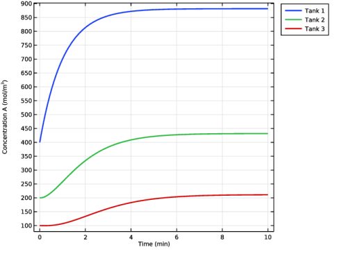
In the Settings window for Global, click Replace Expression in the upper-right corner of the y-Axis Data section. From the menu, choose Component 1 (comp1) > Reaction Engineering > tank1.c_A - Concentration - mol/m³.
3
Click Add Expression in the upper-right corner of the y-Axis Data section. From the menu, choose Component 1 (comp1) > Reaction Engineering 2 > tank2.c_A - Concentration - mol/m³.
4
Click Add Expression in the upper-right corner of the y-Axis Data section. From the menu, choose Component 1 (comp1) > Reaction Engineering 3 > tank3.c_A - Concentration - mol/m³.
5
Locate the x-Axis Data section. From the Parameter list, choose Expression.
6
In the Expression text field, type t.
7
From the Unit list, choose min.
8
Click to expand the Coloring and Style section. From the Width list, choose 2.
9
Click to expand the Legends section. From the Legends list, choose Manual.
10
11
In the Open Loop toolbar, click  Plot.
12
Click the  Zoom Extents button in the Graphics toolbar.
Component 1 (comp1)
Set up the feedback control to model the closed loop system using the Global ODEs and PDEs interface and some variables.
Add Physics
1
In the Home toolbar, click  Add Physics to open the Add Physics window.
2
Go to the Add Physics window.
3
In the tree, select Mathematics > ODE and DAE Interfaces > Global ODEs and DAEs (ge).
4
Click the Add to Component 1 button in the window toolbar.
5
In the Home toolbar, click  Add Physics to close the Add Physics window.
Global ODEs and DAEs (ge)
Global Equations 1 (ODE7)
1
In the Model Builder window, under Component 1 (comp1) > Global ODEs and DAEs (ge) click Global Equations 1 (ODE7).
2
In the Settings window for Global Equations, locate the Global Equations section.
3
4
Locate the Units section. Click  Define Dependent Variable Unit.
5
In the Dependent variable quantity table, enter the following settings:
6
Click  Select Source Term Quantity.
7
In the Physical Quantity dialog, type concentration in the text field.
8
In the tree, select General > Concentration (mol/m^3).
9
Definitions
Variables 1
1
In the Model Builder window, under Component 1 (comp1) right-click Definitions and choose Variables.
2
In the Settings window for Variables, locate the Variables section.
3
Study 1
In the Study toolbar, click  Compute.
Close Loop
1
In the Model Builder window, under Study 1 > Solver Configurations click Solution 1 (sol1).
2
In the Settings window for Solution, type Close Loop in the Label text field.
Follow the steps below to plot the concentration of species A in all three tanks and at the inlet for the closed loop system.
Results
Closed Loop
1
In the Model Builder window, right-click Open Loop and choose Duplicate.
2
In the Settings window for 1D Plot Group, type Closed Loop in the Label text field.
3
Locate the Data section. From the Dataset list, choose Study 1/Close Loop (sol1).
4
Click to expand the Title section. From the Title type list, choose None.
5
Locate the Legend section. From the Layout list, choose Outside graph axis area.
Global 1
1
In the Model Builder window, expand the Closed Loop node, then click Global 1.
2
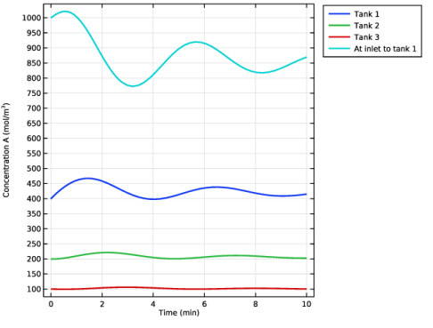
In the Settings window for Global, click Add Expression in the upper-right corner of the y-Axis Data section. From the menu, choose Component 1 (comp1) > Definitions > Variables > cinlet_A - Inlet concentration - mol/m³.
3
Locate the Legends section. In the table, enter the following settings:
4
In the Closed Loop toolbar, click  Plot.
5
Click the  Zoom Extents button in the Graphics toolbar.