|
|
|
|
1
|
|
2
|
|
3
|
Click
|
|
4
|
Browse to the model’s Application Libraries folder and double-click the file stirred_tank_adc_production_process_parameters.txt.
|
|
5
|
|
1
|
|
2
|
|
3
|
Click
|
|
4
|
Browse to the model’s Application Libraries folder and double-click the file stirred_tank_adc_production_geometry_parameters.txt.
|
|
5
|
|
1
|
|
2
|
Go to the Add Physics window.
|
|
3
|
|
4
|
Click the Add to Ideal Semibatch Reactor button in the window toolbar.
|
|
5
|
|
1
|
|
2
|
|
3
|
|
4
|
|
1
|
|
2
|
|
3
|
|
4
|
Click Apply.
|
|
5
|
|
1
|
|
2
|
|
3
|
|
1
|
|
2
|
|
3
|
|
1
|
|
2
|
|
3
|
|
1
|
|
2
|
|
3
|
|
4
|
Click Apply.
|
|
5
|
|
1
|
|
2
|
|
3
|
|
1
|
|
2
|
|
3
|
|
4
|
Click Apply.
|
|
5
|
|
1
|
|
2
|
|
3
|
|
1
|
|
2
|
|
3
|
|
4
|
Locate the Volumetric Species Initial Values section. In the table, enter the following settings:
|
|
1
|
|
2
|
|
3
|
|
4
|
Click to expand the Smoothing section. In the Size of transition zone text field, type t_transitionZone.
|
|
1
|
|
2
|
|
3
|
|
4
|
Locate the Definition section. In the Expression text field, type v_feed*(t<t_feed+t_transitionZone)*step1(t).
|
|
5
|
|
6
|
|
8
|
Locate the Plot Parameters section. In the table, enter the following settings:
|
|
1
|
|
2
|
|
3
|
|
4
|
Locate the Feed Inlet Concentration section. In the table, enter the following settings:
|
|
1
|
|
2
|
Go to the Add Study window.
|
|
3
|
|
4
|
Click the Add Study button in the window toolbar.
|
|
5
|
|
1
|
|
2
|
|
3
|
|
4
|
|
5
|
|
1
|
|
2
|
|
3
|
|
4
|
From the list, choose Turbulent Flow, Diluted Species.
|
|
5
|
|
6
|
|
1
|
|
2
|
|
1
|
|
2
|
Browse to the model’s Application Libraries folder and double-click the file stirred_tank_adc_production_geom_sequence.mph.
|
|
3
|
|
1
|
|
2
|
In the Settings window for Explicit Selection, in the Graphics window toolbar, click
|
|
3
|
|
4
|
|
5
|
On the object fin, select Boundaries 13, 14, 17, 18, 43, 45, 51, and 67 only.
|
|
1
|
|
2
|
|
3
|
|
4
|
|
5
|
On the object fin, select Edges 150–153, 155, 156, 158, 159, 161, 162, 170, 173, 175, 176, 178, 179, 181, 182, 184, 186, 188, 193, 195, 198, 199, 201, 206, 208, 210, 212, 236–240, 243–248, 251–255, 257–260, 265, 266, 269, 272, 276, 277, 279, 280, 282, and 283 only.
|
|
6
|
|
1
|
|
2
|
In the Settings window for Explicit Selection, type Explicit Selection 3: Source (Mesh) in the Label text field.
|
|
3
|
|
4
|
On the object fin, select Boundaries 73–80, 109–112, 114, and 116–118 only.
|
|
1
|
|
2
|
In the Settings window for Explicit Selection, type Explicit Selection 4: Destination (Mesh) in the Label text field.
|
|
3
|
|
4
|
On the object fin, select Boundaries 21–28, 55–58, 61, 63, 65, and 66 only.
|
|
1
|
|
2
|
In the Settings window for Explicit Selection, type Explicit Selection 5: Inside Glass Wall Boundary (Mesh) in the Label text field.
|
|
3
|
|
4
|
On the object fin, select Boundaries 9–12, 31, 32, 41, 42, 48, 50, 53, 56, and 69 only.
|
|
1
|
Go to the Add Material window.
|
|
2
|
|
3
|
Click the Add to Component button in the window toolbar.
|
|
4
|
|
1
|
|
2
|
|
1
|
|
2
|
|
3
|
|
4
|
|
5
|
|
6
|
|
7
|
|
8
|
|
1
|
In the Model Builder window, expand the Space-Dependent Reactor (comp2) > Transport of Diluted Species (tds) node, then click Fluid 1.
|
|
2
|
|
3
|
|
1
|
|
2
|
|
3
|
|
4
|
Locate the Species Source section. In the [[dot]]qp,cDrug text field, type comp1.feedRate(t)*c_feed_Drug.
|
|
1
|
|
2
|
|
3
|
|
4
|
|
1
|
In the Model Builder window, expand the Space-Dependent Reactor (comp2) > Turbulent Flow, k-ε (spf) > Fluid Properties 1 node, then click Fluid Properties 1.
|
|
2
|
|
3
|
|
1
|
|
1
|
|
2
|
|
3
|
|
1
|
|
2
|
|
3
|
From the list, choose User-controlled mesh.
|
|
1
|
|
2
|
|
3
|
|
4
|
Click the Custom button.
|
|
5
|
|
6
|
|
1
|
|
2
|
|
3
|
|
4
|
|
5
|
Locate the Element Size Parameters section.
|
|
6
|
|
7
|
|
1
|
|
2
|
|
3
|
|
4
|
|
5
|
Locate the Element Size Parameters section.
|
|
6
|
|
7
|
|
8
|
|
9
|
|
10
|
|
1
|
|
2
|
|
3
|
|
4
|
|
5
|
|
6
|
|
7
|
Click the Custom button.
|
|
8
|
Locate the Element Size Parameters section.
|
|
9
|
|
10
|
|
11
|
|
12
|
|
13
|
|
1
|
|
2
|
|
3
|
|
4
|
|
5
|
|
6
|
Click the Custom button.
|
|
7
|
Locate the Element Size Parameters section.
|
|
8
|
|
9
|
|
10
|
|
11
|
|
12
|
|
1
|
|
2
|
|
3
|
|
4
|
From the Selection list, choose Stirrer Blade Short Surfaces (Straight Blade Bottom Fitted Impeller 1).
|
|
5
|
|
6
|
Locate the Element Size Parameters section.
|
|
7
|
|
1
|
|
2
|
|
3
|
|
4
|
Locate the Second Entity Group section. From the Selection list, choose Explicit Selection 4: Destination (Mesh).
|
|
1
|
|
2
|
|
3
|
|
4
|
Click to select the
|
|
1
|
|
2
|
|
3
|
|
4
|
|
5
|
Click
|
|
1
|
In the Model Builder window, expand the Boundary Layers 1 node, then click Boundary Layer Properties 1.
|
|
3
|
|
1
|
|
2
|
|
3
|
Click
|
|
4
|
|
5
|
|
6
|
|
1
|
|
2
|
In the Settings window for Point Probe, type Probe 2: Top of Tank Opposite Stirrer in the Label text field.
|
|
3
|
|
1
|
|
2
|
|
3
|
|
4
|
|
1
|
In the Model Builder window, expand the Probe 3: Center of Tank Near Cone node, then click Point Probe Expression 1 (ppb1).
|
|
2
|
|
3
|
|
1
|
|
2
|
In the Settings window for Domain Point Probe, type Probe 4: Between Wall and Rotary Domain in the Label text field.
|
|
3
|
|
1
|
|
2
|
Go to the Add Study window.
|
|
3
|
Find the Studies subsection. In the Select Study tree, select Preset Studies for Some Physics Interfaces > Frozen Rotor.
|
|
4
|
Click the Add Study button in the window toolbar.
|
|
1
|
|
2
|
In the Solve for column of the table, under Space-Dependent Reactor (comp2), clear the checkboxes for Chemistry (chem) and Transport of Diluted Species (tds).
|
|
3
|
In the Solve for column of the table, under Space-Dependent Reactor (comp2) > Multiphysics, clear the checkbox for Reacting Flow, Diluted Species 1 (rfd1).
|
|
4
|
|
5
|
Click
|
|
7
|
|
8
|
|
9
|
|
1
|
In the Model Builder window, expand the Results > Frozen Rotor > Velocity (spf) node, then click Velocity (spf).
|
|
2
|
In the Settings window for 3D Plot Group, type Frozen Rotor: Velocity (spf) in the Label text field.
|
|
1
|
|
2
|
|
3
|
|
4
|
|
1
|
In the Model Builder window, expand the Results > Frozen Rotor > Pressure (spf) node, then click Pressure (spf).
|
|
2
|
In the Settings window for 3D Plot Group, type Frozen Rotor: Pressure (spf) in the Label text field.
|
|
1
|
|
2
|
|
3
|
|
4
|
|
1
|
In the Model Builder window, expand the Results > Frozen Rotor > Wall Resolution (spf) node, then click Wall Resolution (spf).
|
|
2
|
In the Settings window for 3D Plot Group, type Frozen Rotor: Wall Resolution (spf) in the Label text field.
|
|
1
|
|
2
|
|
3
|
|
1
|
Go to the Add Study window.
|
|
2
|
|
3
|
Click the Add Study button in the window toolbar.
|
|
4
|
|
1
|
|
2
|
|
3
|
Locate the Physics and Variables Selection section. In the Solve for column of the table, clear the checkbox for Ideal Semibatch Reactor (comp1).
|
|
4
|
In the Solve for column of the table, under Space-Dependent Reactor (comp2), clear the checkboxes for Chemistry (chem) and Transport of Diluted Species (tds).
|
|
5
|
In the Solve for column of the table, under Space-Dependent Reactor (comp2) > Multiphysics, clear the checkbox for Reacting Flow, Diluted Species 1 (rfd1).
|
|
6
|
Click to expand the Values of Dependent Variables section. Find the Initial values of variables solved for subsection. From the Settings list, choose User controlled.
|
|
7
|
|
8
|
|
9
|
|
10
|
|
11
|
|
12
|
|
1
|
|
2
|
|
3
|
|
4
|
|
1
|
In the Model Builder window, expand the Results > Time-Dependent Flow Field > Pressure (spf) node, then click Surface.
|
|
2
|
|
3
|
|
4
|
|
1
|
|
2
|
|
3
|
|
1
|
|
2
|
|
3
|
|
4
|
Drag and drop on Time-Dependent Flow Field.
|
|
1
|
|
2
|
In the Settings window for Table, type Probe Table 1: Time-Dependent Flow Field in the Label text field.
|
|
1
|
|
2
|
|
1
|
In the Model Builder window, under Space-Dependent Reactor (comp2) > Definitions click Probe 1: Feed Point (point1).
|
|
2
|
|
3
|
Click
|
|
1
|
|
2
|
|
3
|
|
1
|
In the Model Builder window, under Space-Dependent Reactor (comp2) > Definitions > Probe 3: Center of Tank Near Cone click Point Probe Expression 1 (ppb1).
|
|
2
|
In the Settings window for Point Probe Expression, click to expand the Table and Window Settings section.
|
|
3
|
|
1
|
In the Model Builder window, expand the Space-Dependent Reactor (comp2) > Definitions > Probe 4: Between Wall and Rotary Domain node, then click Point Probe Expression 1 (ppb2).
|
|
2
|
|
3
|
|
1
|
|
2
|
Go to the Add Study window.
|
|
3
|
|
4
|
Click the Add Study button in the window toolbar.
|
|
5
|
|
1
|
|
2
|
|
3
|
Locate the Physics and Variables Selection section. In the Solve for column of the table, clear the checkbox for Ideal Semibatch Reactor (comp1).
|
|
4
|
Locate the Values of Dependent Variables section. Find the Initial values of variables solved for subsection. From the Settings list, choose User controlled.
|
|
5
|
|
6
|
|
7
|
|
8
|
|
9
|
In the Settings window for Study, type Study 4: Space-Dependent Semibatch Reactor in the Label text field.
|
|
1
|
|
2
|
|
3
|
In the Model Builder window, expand the Study 4: Space-Dependent Semibatch Reactor > Solver Configurations > Solution 4 (sol4) > Dependent Variables 1 node, then click Concentration (comp2.cDrug).
|
|
4
|
|
5
|
|
6
|
|
7
|
In the Model Builder window, under Study 4: Space-Dependent Semibatch Reactor > Solver Configurations > Solution 4 (sol4) > Dependent Variables 1 click Concentration (comp2.cmAb).
|
|
8
|
|
9
|
|
10
|
|
1
|
In the Model Builder window, collapse the Study 4: Space-Dependent Semibatch Reactor > Solver Configurations > Solution 4 (sol4) > Dependent Variables 1 node.
|
|
2
|
In the Model Builder window, under Study 4: Space-Dependent Semibatch Reactor > Solver Configurations > Solution 4 (sol4) click Time-Dependent Solver 1.
|
|
3
|
|
4
|
|
5
|
|
6
|
In the Settings window for Study, type Study 4: Space-Dependent Semibatch Reactor in the Label text field.
|
|
7
|
|
8
|
|
1
|
|
2
|
|
3
|
Locate the Data section. From the Dataset list, choose Study 4: Space-Dependent Semibatch Reactor/Solution 4 (8) (sol4).
|
|
4
|
|
5
|
|
6
|
|
7
|
|
8
|
|
9
|
Clear the Plot dataset edges checkbox.
|
|
10
|
|
11
|
Select the Show units checkbox.
|
|
12
|
|
13
|
|
14
|
|
15
|
|
1
|
|
2
|
|
3
|
|
4
|
|
5
|
|
6
|
|
1
|
|
2
|
|
3
|
|
4
|
|
1
|
|
2
|
|
3
|
|
4
|
|
1
|
|
1
|
|
2
|
|
3
|
|
4
|
|
1
|
|
2
|
|
3
|
|
4
|
|
1
|
|
2
|
|
3
|
|
1
|
|
2
|
|
3
|
|
4
|
|
5
|
|
6
|
|
7
|
|
8
|
|
1
|
|
2
|
|
3
|
|
4
|
|
5
|
|
6
|
|
7
|
|
1
|
|
2
|
|
3
|
|
1
|
In the Model Builder window, under Results > 2s, Ctrl-click to select Surface 1: Tank, Surface 2: Stirrer, and (a).
|
|
2
|
Right-click and choose Duplicate.
|
|
1
|
|
2
|
|
1
|
|
2
|
|
3
|
|
1
|
|
2
|
|
3
|
|
4
|
|
1
|
|
2
|
Click the Zoom Box button on the Graphics toolbar and then use the mouse to zoom in. Adjust the view according to your preferences.
|
|
1
|
|
2
|
|
3
|
|
1
|
|
2
|
|
3
|
|
1
|
|
2
|
|
3
|
Select the Manual color range checkbox.
|
|
4
|
|
5
|
|
1
|
|
2
|
|
3
|
|
1
|
|
2
|
Right-click and choose Group.
|
|
1
|
|
2
|
|
3
|
|
1
|
In the Model Builder window, expand the Results > Concentration mAbDrug > 2s 1 node, then click Slice 1.
|
|
2
|
|
3
|
|
4
|
|
1
|
|
2
|
|
3
|
|
4
|
|
1
|
In the Model Builder window, expand the Results > Concentration mAbDrug > 4s 1 node, then click Slice 1.
|
|
2
|
|
3
|
|
4
|
|
1
|
|
2
|
|
3
|
|
4
|
|
1
|
In the Model Builder window, expand the Results > Concentration mAbDrug > 8s 1 node, then click Slice 1.
|
|
2
|
|
3
|
|
4
|
|
5
|
|
6
|
|
1
|
|
2
|
|
3
|
|
4
|
|
1
|
In the Model Builder window, expand the Results > Concentration mAbDrug > 16s 1 node, then click Slice 1.
|
|
2
|
|
3
|
|
4
|
|
5
|
|
6
|
|
1
|
|
2
|
|
3
|
|
4
|
|
1
|
|
2
|
Go to the Result Templates window.
|
|
3
|
In the tree, select Study 4: Space-Dependent Semibatch Reactor/Solution 4 (8) (sol4) > Turbulent Flow, k-ε > Velocity Streamlines (spf).
|
|
4
|
Click the Add Result Template button in the window toolbar.
|
|
1
|
|
2
|
|
3
|
|
4
|
|
5
|
|
6
|
Locate the Coloring and Style section. Find the Line style subsection. From the Type list, choose Tube.
|
|
7
|
|
8
|
|
9
|
|
10
|
|
1
|
|
2
|
|
3
|
|
1
|
In the Model Builder window, under Results > Concentration mAbDrug2 > 16s 1.1, Ctrl-click to select Surface 1: Tank and Surface 2: Stirrer.
|
|
2
|
Right-click and choose Copy.
|
|
1
|
In the Model Builder window, under Results > Concentration mAbDrug2 right-click Velocity Streamlines (spf) and choose Paste Multiple Items.
|
|
2
|
|
3
|
Clear the Plot dataset edges checkbox.
|
|
4
|
|
1
|
|
2
|
|
3
|
|
1
|
|
2
|
|
3
|
|
4
|
|
5
|
Locate the Expressions section. In the table, enter the following settings:
|
|
6
|
|
1
|
Go to the Evaluation Group 1 window.
|
|
2
|
Click the Table Graph button in the window toolbar.
|
|
1
|
|
2
|
|
3
|
|
4
|
|
5
|
|
6
|
|
1
|
|
2
|
|
3
|
|
4
|
|
6
|
Click to expand the Coloring and Style section. Find the Line style subsection. From the Line list, choose Cycle.
|
|
7
|
|
8
|
|
1
|
|
2
|
|
3
|
Locate the Plot Settings section.
|
|
4
|
|
5
|
|
6
|
|
1
|
|
2
|
Drag and drop above Table Graph 1.
|
|
3
|
|
1
|
|
2
|
|
3
|
|
4
|
|
5
|
Locate the Expressions section. In the table, enter the following settings:
|
|
6
|
|
1
|
|
2
|
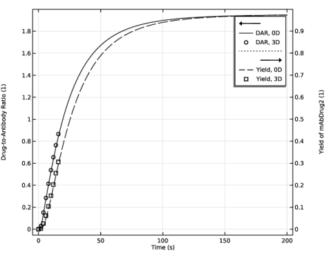
In the Settings window for 1D Plot Group, type Drug-to-Antibody Ratio and Yield in the Label text field.
|
|
1
|
|
2
|
|
3
|
|
5
|
|
6
|
|
7
|
Clear the Solution checkbox.
|
|
8
|
Clear the Expression checkbox.
|
|
1
|
|
2
|
|
3
|
Locate the y-Axis Data section. In the table, enter the following settings:
|
|
4
|
Locate the Coloring and Style section. Find the Line style subsection. From the Line list, choose Dashed.
|
|
1
|
|
2
|
|
3
|
|
4
|
|
5
|
|
6
|
Locate the Coloring and Style section. Find the Line style subsection. From the Line list, choose None.
|
|
7
|
|
8
|
|
9
|
|
10
|
|
11
|
|
12
|
Clear the Headers checkbox.
|
|
1
|
|
2
|
|
3
|
|
4
|
Locate the Coloring and Style section. Find the Line markers subsection. From the Marker list, choose Square.
|
|
1
|
|
2
|
|
3
|
Select the Two y-axes checkbox.
|
|
4
|
|
5
|
|
6
|
Select the Secondary y-axis label checkbox.
|
|
7
|