|
|
|


|
1
|
|
2
|
|
3
|
Click Add.
|
|
4
|
Click
|
|
5
|
In the Select Study tree, select Preset Studies for Selected Physics Interfaces > Stationary Plug Flow.
|
|
6
|
Click
|
|
1
|
|
2
|
|
3
|
Click
|
|
4
|
Browse to the model’s Application Libraries folder and double-click the file polymerization_multijet_parameters.txt.
|
|
1
|
In the Model Builder window, under Component 1 (comp1) right-click Definitions and choose Variables.
|
|
2
|
|
1
|
|
2
|
|
3
|
|
4
|
|
5
|
|
1
|
|
2
|
|
3
|
|
4
|
Click Apply.
|
|
5
|
|
6
|
|
7
|
|
8
|
Locate the Reaction Thermodynamic Properties section. From the Enthalpy of reaction list, choose User defined.
|
|
9
|
|
1
|
|
2
|
|
3
|
|
4
|
|
1
|
|
2
|
|
3
|
|
4
|
|
1
|
|
2
|
|
3
|
|
4
|
|
5
|
|
6
|
|
1
|
|
2
|
|
3
|
|
4
|
|
1
|
|
2
|
|
3
|
|
4
|
|
1
|
|
2
|
|
3
|
|
4
|
Click Apply.
|
|
5
|
|
6
|
|
7
|
|
8
|
|
9
|
|
10
|
Locate the Reaction Thermodynamic Properties section. From the Enthalpy of reaction list, choose User defined.
|
|
11
|
|
1
|
|
2
|
|
3
|
|
4
|
|
1
|
|
2
|
|
3
|
|
4
|
Locate the Volumetric Species Initial Values section. In the table, enter the following settings:
|
|
1
|
|
2
|
|
3
|
|
4
|
|
1
|
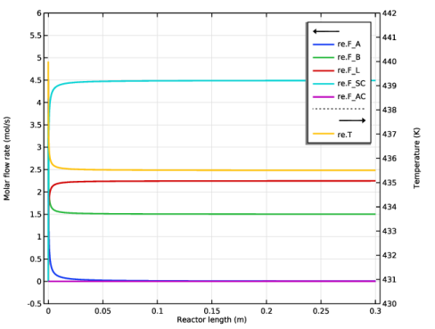
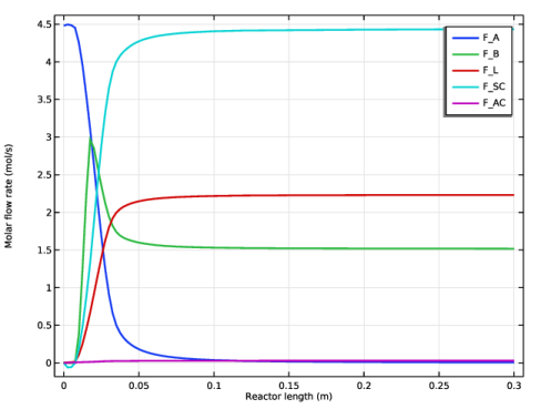
In the Settings window for 1D Plot Group, type Plug Flow: Flow Rate and Temperature in the Label text field.
|
|
2
|
|
3
|
|
4
|
Select the Two y-axes checkbox.
|
|
5
|
|
1
|
In the Model Builder window, expand the Plug Flow: Flow Rate and Temperature node, then click Global 1.
|
|
2
|
|
4
|
|
5
|
|
6
|
|
1
|
|
2
|
|
4
|
|
5
|
|
6
|
|
1
|
|
2
|
|
3
|
|
4
|
|
5
|
|
6
|
|
7
|
|
8
|
|
9
|
|
1
|
|
2
|
|
3
|
Find the Chemical species transport subsection. From the list, choose Nonisothermal Reacting Flow: New.
|
|
4
|
From the list, choose Turbulent Flow.
|
|
5
|
|
1
|
|
2
|
|
3
|
Browse to the model’s Application Libraries folder and double-click the file polymerization_multijet_geom_sequence.mph.
|
|
4
|
|
1
|
|
2
|
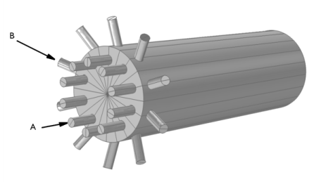
On the object fin, select Domain 4 only.
|
|
1
|
|
2
|
On the object mcd1, select Boundary 11 only.
|
|
1
|
|
2
|
|
3
|
|
4
|
|
1
|
In the Model Builder window, expand the Component 2 (comp2) > Turbulent Flow, k-ε (spf) node, then click Initial Values 1.
|
|
2
|
|
3
|
|
4
|
|
1
|
|
1
|
|
3
|
|
4
|
From the list, choose Fully developed flow.
|
|
5
|
|
1
|
|
1
|
|
2
|
|
3
|
|
4
|
|
5
|
Click to expand the Calculate Transport Properties section. From the Heat capacity list, choose User defined.
|
|
6
|
|
7
|
|
8
|
|
9
|
|
1
|
In the Model Builder window, under Component 2 (comp2) click Transport of Concentrated Species (tcs).
|
|
2
|
In the Settings window for Transport of Concentrated Species, locate the Transport Mechanisms section.
|
|
3
|
|
4
|
|
1
|
In the Model Builder window, expand the Transport of Concentrated Species (tcs) node, then click Fluid 1.
|
|
2
|
|
3
|
|
4
|
|
5
|
|
6
|
|
7
|
|
8
|
|
9
|
|
1
|
|
2
|
|
3
|
|
4
|
|
5
|
|
6
|
|
7
|
|
1
|
|
3
|
|
4
|
|
5
|
|
6
|
|
7
|
|
8
|
|
9
|
|
1
|
|
3
|
|
4
|
|
5
|
|
6
|
|
7
|
|
8
|
|
9
|
|
1
|
|
1
|
|
1
|
|
3
|
|
4
|
|
5
|
Clear the Mass transfer to other phases checkbox.
|
|
1
|
In the Model Builder window, under Component 2 (comp2) > Heat Transfer in Fluids (ht) click Initial Values 1.
|
|
2
|
|
3
|
|
1
|
|
3
|
|
4
|
|
1
|
|
1
|
|
1
|
|
2
|
|
3
|
|
1
|
|
2
|
|
3
|
|
1
|
|
2
|
|
3
|
|
5
|
|
6
|
|
1
|
|
2
|
|
3
|
|
1
|
|
2
|
|
3
|
|
4
|
|
5
|
|
1
|
|
2
|
|
3
|
|
1
|
|
3
|
|
4
|
|
5
|
|
6
|
Click
|
|
1
|
|
2
|
|
3
|
In the Solve for column of the table, under Component 2 (comp2), clear the checkboxes for Transport of Concentrated Species (tcs) and Heat Transfer in Fluids (ht).
|
|
4
|
In the Solve for column of the table, under Component 2 (comp2) > Multiphysics, clear the checkbox for Reacting Flow 1 (nirf1).
|
|
1
|
|
2
|
|
3
|
|
4
|
Clear the Generate default plots checkbox.
|
|
5
|
|
1
|
|
2
|
|
3
|
|
4
|
|
5
|
|
6
|
|
7
|
|
8
|
|
9
|
|
10
|
Click
|
|
1
|
|
2
|
|
3
|
|
4
|
|
5
|
|
6
|
|
1
|
|
2
|
|
3
|
|
4
|
|
5
|
Click
|
|
1
|
|
2
|
|
3
|
|
4
|
|
5
|
Click
|
|
6
|
|
1
|
|
2
|
|
3
|
|
4
|
|
1
|
|
2
|
|
3
|
|
4
|
|
5
|
|
1
|
|
2
|
|
1
|
|
1
|
|
2
|
|
3
|
|
1
|
|
2
|
|
3
|
|
4
|
|
5
|
|
6
|
|
1
|
|
2
|
|
1
|
|
2
|
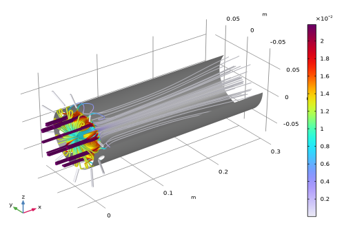
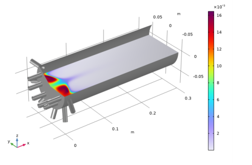
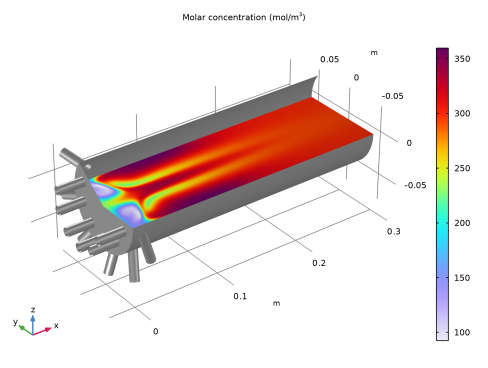
In the Settings window for Slice, click Replace Expression in the upper-right corner of the Expression section. From the menu, choose Component 2 (comp2) > Transport of Concentrated Species > Species wA > tcs.c_wA - Molar concentration - mol/m³.
|
|
1
|
|
2
|
|
3
|
|
4
|
|
5
|
|
6
|
|
7
|
|
8
|
|
1
|
|
2
|
|
1
|
|
2
|
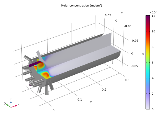
In the Settings window for Slice, click Replace Expression in the upper-right corner of the Expression section. From the menu, choose Component 2 (comp2) > Transport of Concentrated Species > Species wL > tcs.c_wL - Molar concentration - mol/m³.
|
|
3
|
|
1
|
|
2
|
|
3
|
|
1
|
|
2
|
|
1
|
|
2
|
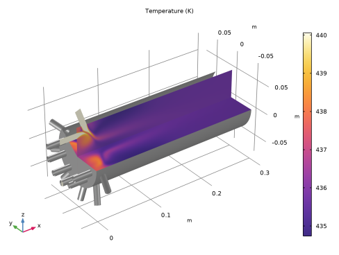
In the Settings window for Slice, click Replace Expression in the upper-right corner of the Expression section. From the menu, choose Component 2 (comp2) > Heat Transfer in Fluids > Temperature > T - Temperature - K.
|
|
3
|
|
1
|
|
2
|
In the Settings window for Slice, click Replace Expression in the upper-right corner of the Expression section. From the menu, choose Component 2 (comp2) > Heat Transfer in Fluids > Temperature > T - Temperature - K.
|
|
3
|
|
4
|
|
1
|
|
2
|
|
3
|
Select the Additional parallel planes checkbox.
|
|
4
|
|
1
|
|
2
|
|
3
|
|
1
|
|
2
|
|
4
|
|
1
|
|
2
|
Select the Evaluate each plane separately checkbox.
|
|
3
|
Click Replace Expression in the upper-right corner of the Expressions section. From the menu, choose Component 2 (comp2) > Transport of Concentrated Species > Species wA > Fluxes > Total flux - kg/(m²·s) > tcs.tflux_wAx - Total flux, x-component.
|
|
4
|
Locate the Expressions section. In the table, enter the following settings:
|
|
5
|
|
1
|
|
2
|
|
1
|
|
2
|
|
1
|
|
2
|
|
1
|
|
2
|
|
1
|
|
2
|
|
3
|
Select the Transpose checkbox.
|
|
4
|
|
5
|
|
1
|
Go to the Evaluation Group 1 window.
|
|
2
|
Click the Table Graph button in the window toolbar.
|
|
1
|
|
2
|
|
1
|
|
2
|
|
3
|
|
4
|
|
5
|
|
6
|
|
1
|
|
2
|
|
3
|
|
4
|
|
1
|
|
2
|
|
3
|
|
4
|
|
5
|
|
6
|
|
1
|
|
2
|
|
3
|
|
4
|
Locate the Coloring and Style section. Find the Line style subsection. From the Type list, choose Tube.
|
|
5
|
|
1
|
|
2
|
|
3
|
|
4
|
|
5
|
|
1
|
|
2
|
|
1
|
|
2
|
|
3
|
|
4
|
|
1
|
|
1
|
|
2
|
|
1
|
|
2
|
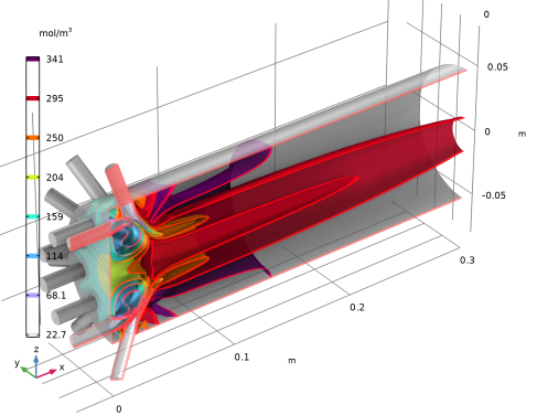
In the Settings window for 3D Plot Group, type Concentration, L (Isosurface) in the Label text field.
|
|
3
|
|
4
|
|
5
|
|
1
|
|
2
|
In the Settings window for Isosurface, click Replace Expression in the upper-right corner of the Expression section. From the menu, choose Component 2 (comp2) > Transport of Concentrated Species > Species wL > tcs.c_wL - Molar concentration - mol/m³.
|
|
3
|
|
4
|
|
5
|
|
6
|
|
1
|
|
2
|
|
3
|
|
4
|
Clear the Plot dataset edges checkbox.
|
|
5
|
|
6
|
|
7
|
|
8
|
|
9
|
|
10
|
From the gizmo context menu, select Align to y-Axis.
|
|
11
|
From the gizmo context menu, select Invert Clipping.
|
|
12
|
|
1
|
|
2
|
|
3
|
|
1
|
|
2
|
|
3
|
|
4
|
|
5
|
|
1
|
|
2
|
|
3
|
|
1
|
|
2
|
|
3
|
|
4
|
|
5
|
|
1
|
|
2
|
|
3
|
|
4
|
|
1
|
|
2
|
Click
|
|
1
|
|
2
|
|
3
|
|
4
|
|
5
|
|
6
|
|
7
|
Click
|
|
1
|
|
3
|
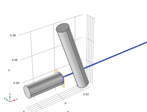
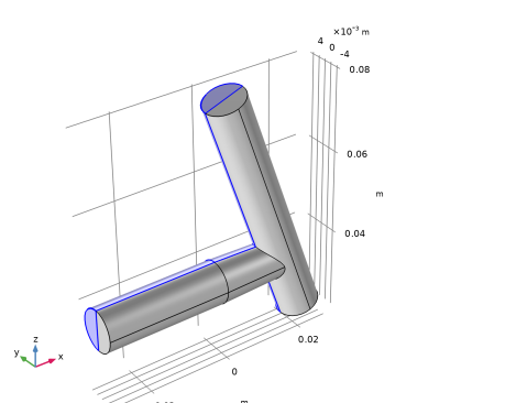
Select the object cyl1 only.
|
|
4
|
|
5
|
|
6
|
|
7
|
|
8
|
|
9
|
Click
|
|
1
|
|
2
|
|
3
|
|
4
|
|
5
|
|
6
|
|
7
|
|
8
|
Click
|
|
1
|
|
2
|
|
3
|
|
5
|
Click to expand the Scales section. In the table, enter the following settings:
|
|
6
|
Click
|
|
1
|
|
2
|
Click in the Graphics window and then press Ctrl+A to select both objects.
|
|
3
|
|
4
|
Clear the Keep interior boundaries checkbox.
|
|
5
|
Click
|
|
1
|
|
2
|
|
3
|
|
1
|
|
2
|
Select the object uni1 only.
|
|
3
|
|
4
|
|
5
|
Click
|
|
6
|
|
7
|
|
1
|
|
2
|
|
3
|
|
4
|
Click
|
|
1
|
|
2
|
|
3
|
|
4
|
|
5
|
|
6
|
Click
|
|
1
|
In the Model Builder window, under Component 1 (comp1) > Geometry 1 right-click Work Plane 2 (wp2) and choose Extrude.
|
|
2
|
|
4
|
Click
|
|
1
|
|
2
|