|
|
|
|
1
|
|
2
|
|
3
|
Click Add.
|
|
4
|
|
5
|
Click Add.
|
|
6
|
|
7
|
In the Concentrations (mol/m³) table, enter the following settings:
|
|
8
|
|
9
|
Click Add.
|
|
10
|
|
11
|
Click Add.
|
|
12
|
|
13
|
Click
|
|
14
|
|
15
|
Click
|
|
1
|
|
2
|
|
3
|
Click
|
|
4
|
Browse to the model’s Application Libraries folder and double-click the file optimal_cooling_parameters.txt.
|
|
1
|
|
2
|
|
4
|
Click
|
|
1
|
|
2
|
|
3
|
|
1
|
|
2
|
|
1
|
|
2
|
Go to the Add Material window.
|
|
3
|
|
4
|
Click the Add to Component button in the window toolbar.
|
|
5
|
|
1
|
|
2
|
|
3
|
|
1
|
|
2
|
|
3
|
|
4
|
Click Apply.
|
|
5
|
|
6
|
|
7
|
|
8
|
Locate the Reaction Thermodynamic Properties section. From the Enthalpy of reaction list, choose User defined.
|
|
9
|
|
1
|
|
2
|
|
3
|
|
1
|
|
2
|
|
3
|
|
1
|
|
2
|
|
3
|
|
4
|
Click Apply.
|
|
5
|
|
6
|
|
7
|
|
8
|
Locate the Reaction Thermodynamic Properties section. From the Enthalpy of reaction list, choose User defined.
|
|
9
|
|
1
|
|
2
|
|
3
|
Clear the Enable formula checkbox.
|
|
4
|
|
1
|
|
2
|
|
3
|
|
4
|
Click Apply.
|
|
5
|
|
6
|
|
7
|
|
8
|
|
9
|
Find the Bulk species subsection. From the Species solved for list, choose Transport of Diluted Species.
|
|
1
|
In the Model Builder window, under Component 1 (comp1) > Transport of Diluted Species (tds) click Fluid 1.
|
|
2
|
|
3
|
|
4
|
|
5
|
|
6
|
|
1
|
|
3
|
|
4
|
|
1
|
|
1
|
|
3
|
|
4
|
|
1
|
|
2
|
In the Settings window for Heat Transfer in Fluids, type Heat Transfer in Fluids - Reactor in the Label text field.
|
|
1
|
In the Model Builder window, under Component 1 (comp1) > Heat Transfer in Fluids - Reactor (ht) click Fluid 1.
|
|
2
|
|
3
|
|
1
|
|
3
|
|
4
|
|
1
|
|
1
|
|
3
|
|
4
|
|
1
|
|
2
|
In the Settings window for Heat Transfer in Fluids, type Heat Transfer in Fluids - Cooling jacket in the Label text field.
|
|
1
|
In the Model Builder window, under Component 1 (comp1) > Heat Transfer in Fluids - Cooling jacket (ht2) click Fluid 1.
|
|
2
|
|
3
|
|
1
|
|
3
|
|
4
|
|
1
|
|
1
|
|
3
|
|
4
|
|
1
|
|
2
|
|
3
|
|
4
|
Click
|
|
1
|
|
2
|
|
1
|
In the Model Builder window, under Study 1 > Solver Configurations click Solution 1 - Copy 1 (sol2).
|
|
2
|
|
1
|
|
2
|
|
3
|
|
4
|
|
5
|
Locate the Legends section. Find the Include in automatic mode subsection. Select the Label checkbox.
|
|
6
|
Clear the Point checkbox.
|
|
7
|
Clear the Solution checkbox.
|
|
8
|
Clear the Headers checkbox.
|
|
1
|
|
2
|
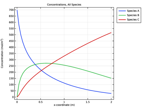
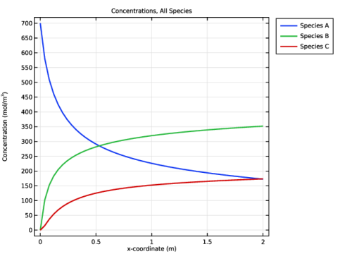
In the Settings window for 1D Plot Group, type Concentrations for Tj_in=400K in the Label text field.
|
|
3
|
|
4
|
Locate the Plot Settings section.
|
|
5
|
|
6
|
Click to expand the Style Configuration section. From the Configuration list, choose Graph Plot Style 1.
|
|
7
|
|
8
|
|
1
|
|
2
|
|
3
|
|
4
|
|
1
|
|
2
|
|
3
|
|
4
|
Click to expand the Coloring and Style section. Click to expand the Legends section. Select the Show legends checkbox.
|
|
1
|
|
2
|
|
3
|
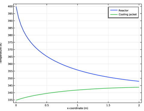
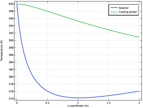
Click Replace Expression in the upper-right corner of the y-Axis Data section. From the menu, choose Component 1 (comp1) > Heat Transfer in Fluids - Cooling jacket > Temperature > Tj - Temperature - K.
|
|
4
|
|
1
|
|
2
|
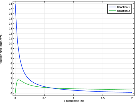
In the Settings window for 1D Plot Group, type Production Rates for Tj_in=400K in the Label text field.
|
|
3
|
|
4
|
|
1
|
In the Model Builder window, expand the Production Rates for Tj_in=400K node, then click Line Graph 1.
|
|
2
|
|
3
|
|
4
|
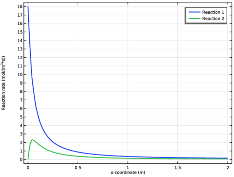
Click Replace Expression in the upper-right corner of the y-Axis Data section. From the menu, choose Component 1 (comp1) > Chemistry > chem.r_1 - Reaction rate - mol/(m³·s).
|
|
5
|
|
1
|
|
2
|
|
3
|
Click Replace Expression in the upper-right corner of the y-Axis Data section. From the menu, choose Component 1 (comp1) > Chemistry > chem.r_2 - Reaction rate - mol/(m³·s).
|
|
4
|
|
1
|
|
2
|
|
3
|
|
4
|
Locate the Objective Function section. In the table, enter the following settings:
|
|
5
|
|
6
|
|
8
|
|
9
|
|
10
|
Clear the Generate default plots checkbox.
|
|
11
|
|
1
|
|
2
|
In the Settings window for 1D Plot Group, type Concentrations for Optimized Tj_in in the Label text field.
|
|
3
|
|
4
|
|
1
|
|
2
|
In the Settings window for 1D Plot Group, type Temperature Tj_in for Optimized Tj_in in the Label text field.
|
|
3
|
|
4
|
|
1
|
|
2
|
In the Settings window for 1D Plot Group, type Production Rates for Optimized Tj_in in the Label text field.
|
|
3
|
|
4
|