|
|
|

|
1
|
|
2
|
|
3
|
Click Add.
|
|
4
|
Click
|
|
5
|
In the Select Study tree, select Preset Studies for Selected Physics Interfaces > Stationary Plug Flow.
|
|
6
|
Click
|
|
1
|
|
2
|
|
3
|
Click
|
|
4
|
Browse to the model’s Application Libraries folder and double-click the file nonisothermal_plug_flow_parameters.txt.
|
|
1
|
|
2
|
|
3
|
|
4
|
|
5
|
|
1
|
|
2
|
|
3
|
|
4
|
|
5
|
|
6
|
|
1
|
|
2
|
|
3
|
|
1
|
|
2
|
|
3
|
|
4
|
Locate the Volumetric Species Initial Values section. In the table, enter the following settings:
|
|
5
|
|
6
|
In the Settings window for Reaction Engineering, click to expand the CHEMKIN Import for Species Properties section.
|
|
7
|
Click
|
|
8
|
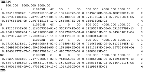
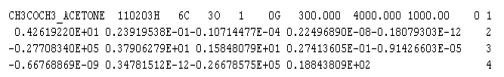
Browse to the model’s Application Libraries folder and double-click the file nonisothermal_plug_flow_thermo.txt.
|
|
9
|
Click
|
|
1
|
In the Model Builder window, under Component 1 (comp1) right-click Definitions and choose Variables.
|
|
2
|
|
1
|
|
2
|
|
3
|
|
4
|
|
1
|
|
2
|
|
1
|
In the Model Builder window, under Study 1 > Solver Configurations click Solution 1 - Copy 1 (sol2).
|
|
2
|
|
1
|
|
2
|
|
3
|
|
1
|
In the Model Builder window, under Study 1 > Solver Configurations click Solution 1 - Copy 1 (sol3).
|
|
2
|
|
1
|
|
2
|
|
3
|
|
1
|
|
2
|
|
3
|
Click
|
|
5
|
|
1
|
In the Model Builder window, under Study 1 > Solver Configurations click Parametric Solutions 1 - Copy 1 (sol8).
|
|
2
|
|
1
|
|
2
|
|
3
|
|
4
|
|
1
|
|
2
|
|
3
|
|
4
|
|
5
|
|
1
|
|
2
|
|
3
|
|
4
|
Locate the Legends section. In the table, enter the following settings:
|
|
5
|
|
1
|
|
2
|
|
3
|
|
1
|
|
2
|
|
3
|
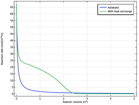
Click Replace Expression in the upper-right corner of the y-Axis Data section. From the menu, choose Component 1 (comp1) > Reaction Engineering > re.r_1 - Reaction rate - mol/(m³·s).
|
|
4
|
|
5
|
|
1
|
|
2
|
|
3
|
|
4
|
Click Replace Expression in the upper-right corner of the y-Axis Data section. From the menu, choose Component 1 (comp1) > Reaction Engineering > re.r_1 - Reaction rate - mol/(m³·s).
|
|
5
|
|
6
|
|
8
|
|
1
|
|
2
|
|
3
|
|
4
|
Locate the Plot Settings section.
|
|
5
|
|
6
|
|
1
|
|
2
|
|
3
|
|
4
|
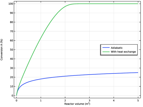
Click Replace Expression in the upper-right corner of the y-Axis Data section. From the menu, choose Component 1 (comp1) > Definitions > Variables > X_A - Conversion, A - 1.
|
|
5
|
|
6
|
|
1
|
|
2
|
|
3
|
|
4
|
Locate the Legends section. In the table, enter the following settings:
|
|
5
|
|
1
|
|
2
|
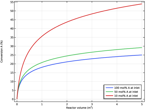
In the Settings window for 1D Plot Group, type Conversion A with inert (re) in the Label text field.
|
|
3
|
|
4
|
Locate the Plot Settings section.
|
|
5
|
Select the x-axis label checkbox. In the associated text field, type Reactor volume (m<sup>3</sup>).
|
|
6
|
|
7
|
|
1
|
|
2
|
|
3
|
|
4
|
Click Replace Expression in the upper-right corner of the y-Axis Data section. From the menu, choose Component 1 (comp1) > Definitions > Variables > X_A - Conversion, A - 1.
|
|
5
|
|
6
|
|
7
|
|
8
|