PDF

NOx and Ammonia Conversion in a Dual-Bed Monolithic Reactor
Introduction
This example illustrates the modeling of a dual bed reactor for exhaust gas treatment in a heavy-duty diesel truck. The reactor consists of two monolithic beds placed in series. In the first bed, selective catalytic reduction (SCR) of NOx (NO and NO2) with ammonia (NH3) occurs. Downstream of this catalytic bed, an ammonia-slip catalyst (ASC) is installed. The ASC bed converts the unreacted ammonia into nitrogen. In both beds there are also undesired side-reactions. The complex chemical kinetics is investigated in detail in Analysis of NOx and Ammonia Conversion Kinetics in a Dual-Bed Plug-Flow Reactor. From that study, where a single monolith channel was modeled, it is clear that temperature plays a central role for the selectivity of the system. The current model is set up in 2D with axi-symmetry to unravel the full space-dependency of the system.
Model Definition
The single channel model in Analysis of NOx and Ammonia Conversion Kinetics in a Dual-Bed Plug-Flow Reactor shows that temperature plays a central role in affecting the optimal dosing of NH3. Because the temperature distribution is sure to vary from channel to channel in monolithic reactor, a space-dependent model is called for.
Model Geometry
The modeled reactor consists of a metal shell that protects and insulates the two catalysts placed inside. Each catalytic bed consists of a monolithic support that is loaded with active catalytic material. These two porous domains are modeled as one material in this model. The catalysts are placed in series, wrapped in a porous supportive mat, and contained in a metal can. The supportive mat protects the catalysts from vibrations and holds them in place. Each monolith consists of reactive channels separated by impermeable walls. The first bed in the reactor is 0.4 m long, and the second bed is 0.06 m long. They are placed with a small gap between. Both beds have a diameter of 0.32 m. The void fraction of the catalyst beds are 0.75. A seal is placed at the inlet of the support mat to prevent erosion of the mat, as well as bypassing of reactive gas through the mat. This seal is included as a boundary condition during simulation, and not a detail in the geometry.
An illustration of the modeled system is found in Figure 1 below.
Figure 1: The exhaust gas passes through the channels in the monolithic beds in the reactor.
The reactor is symmetric in its design which gives the geometry seen in Figure 2 below.
Figure 2: Symmetry reduces the modeling domain.
Model Equations
The present example takes a pseudo-homogeneous approach to model the thousands of channels present in the monolith reactor. No mass is exchanged between channels, so each channel is described by 1D mass-transport equations. Furthermore, assume fully developed laminar flow in the monolith channels, such that the average flow field is proportional to the pressure difference across each bed. The fluid flow transports mass and energy only in the channel direction. The energy equation describes the temperature of the reacting gas in the channels, as well as the conductive heat transfer in the solid parts of the monolith structure. Because the temperature affects not only the reaction kinetics but also the density and viscosity of the reacting gas, the energy equation is what connects the channels in the reactor structure, turning this into a space-dependent model.
Reaction Kinetics
The chemical equations and rate expressions are described in detail in the single channel model Analysis of NOx and Ammonia Conversion Kinetics in a Dual-Bed Plug-Flow Reactor.
Mass Transport
The mass balances describing transport and reaction in the monolith channels are given by diffusion-convection equations at steady state:
(1)
Here Di denotes the diffusion coefficient (SI unit: m2/s), ci is the species concentration (SI unit: mol/m3), and u equals the velocity vector (SI unit: m/s). The term  Ri (SI unit: mol/(m3·s)) corresponds to the species’ rate expression, which is a function of the reaction rates and the reaction stoichiometry.
Mass transport is only allowed in the direction of the channels, corresponding to direction of the z-axis in the 2D-axisymmetric geometry used in this example. For the diffusive transport, this is accomplished by setting the x- and y-components of the diffusivity matrix to zero. The pressure-driven flow in the monolith is also defined in the direction of the z-axis, hereby restricting the convective mass transport to the channel direction. Each monolith channel thus behaves like a 1D plug flow model with included diffusion. These separate channel models are connected through the heat transfer equations for the reactor monolith.
Species concentrations are defined at the reactor inlet boundaries:
At the outlet, use the Outflow condition:
Fluid Flow
The fluid flow in the system is described by the steady-state continuity equation
.
The flow is modeled as compressible, and a porous slip formulation is used. This formulation ensures a smooth transition between regions with different porosity.
The flow of reacting gas through the monoliths is modeled using Darcy’s Law, with the governing equation:
The monolith block is treated as a porous matrix with the effective permeability κ (SI unit: m2). Similarly to the diffusivity, the x- and y-components of the permeability matrix are much lower than that in the axial direction. The density, ρ (SI unit: kg/m3), and viscosity, μ (SI unit: Pa·s), of the gas are assumed to be well represented by the temperature-dependent properties of nitrogen, as only relatively small concentrations of other gases are present.
Pressure conditions are set at the reactor inlet and outlet boundaries.
Heat Transfer
A single temperature equation describing the heat transfer in the porous monolith reactor can be written as
(2)
where ρf (SI unit: kg/m3) is the fluid density, Cpf (SI unit: J/(kg·K)) is the fluid heat capacity, (ρCp)eff (SI unit: J/(m3·K)) is the effective volumetric heat capacity, and keff (SI unit: W/(m·K)) is the effective thermal conductivity. Furthermore, u (SI unit: m/s) is the fluid velocity field, derived by the fluid flow interface. Q (SI unit: W/m3) is the heat source due to exothermic chemical reactions:
Above, Hj is the heat of reaction for reaction j, and rj is the reaction rate for said reaction.
In the stationary case this implies
(3)
The effective conductivity of the solid-fluid system, keff, is related to the conductivity of the solid, ks, and to the conductivity of the fluid, kf, by
Here Θs denotes the solid material’s volume fraction, which is related to the volume fraction of the fluid Θf (or porosity) by
The Heat Transfer interface sets up Equation 3 for a fluid domain. For the solid monolith walls in the reactor, only heat transfer by conduction applies:
(4)
where ks (SI unit: W/(m·K)) is the thermal conductivity for the solid walls. For the extruded monolith material, the thermal conductivity is anisotropic.
The heat transfer in the porous support mat is also described by Equation 3 and Equation 4. Contrary to the monoliths, the support mat has isotropic thermal conductivity. The same is true for the solid metal walls in the reactor.
The temperature is specified at the metal walls and the edge of the support mat in the reactor inlet:
,
and the Inflow condition, that is
is assigned to the inlet of the first catalytic bed. ΔH (SI unit: J/(kg)) is the sensible enthalpy.
At the outlet of the second bed, use the Outflow condition
.
For the external reactor walls, the heat flux through the boundaries is given by
,
where h (SI unit: W/(m2·K)) denotes the heat transfer coefficient, and Tamb (K) equals the ambient temperature.
As mentioned, the temperature affects not only reaction kinetics but also the density and viscosity of the reacting gas. In this way the heat transfer equation connects the channels in the reactor structure.
Thermodynamic and Transport Properties
Accurate thermodynamic data is required as input to energy balance equations, both in the plug flow model and this 2D axisymmetric monolith model (Equation 2). In addition to thermodynamic properties, the model equations also require transport properties to accurately describe the space-dependent reactor model. For instance, the mass transport (Equation 1) needs species specific diffusion coefficients as input.
The Thermodynamics feature provides all necessary properties for this simulation. Different models are available for calculation of thermal and transport properties (see Thermodynamic Models and Theory). The viscosity of the system is calculated based on the Brokaw model. The thermal conductivity and diffusivity are calculated from Kinetic Theory and Fuller–Schettler–Giddings, respectively.
In this model, to simplify the problem, nitrogen is modeled as a solvent. This means that the gas properties are not composition dependent. Another way to speed up the calculations, also used in this model, is to use Generate Material from Thermodynamics. Information about how to efficiently use the Thermodynamics feature is available at Using Thermodynamic Properties.
Results
The system conditions used in this model are the same as those in the single channel plug flow system, described in Analysis of NOx and Ammonia Conversion Kinetics in a Dual-Bed Plug-Flow Reactor. Three engine load cases are investigated, with a fixed ammonia-to-NOx ratio of 1.3.
The three engine load cases result in the following inlet gas conditions:
Figure 3 shows the molar fraction of NH3, NO, and NO2 in the two catalyst beds for the low engine load case. The effect of the radial temperature gradient is clearly visible as the conversion decreases close to the edge. The temperature for the low engine load case is below the optimal temperature for the SCR reactor, see Analysis of NOx and Ammonia Conversion Kinetics in a Dual-Bed Plug-Flow Reactor. The low temperature results in low conversion of both NOx and ammonia.
Figure 3: Molar fraction of ammonia, nitrogen monoxide, and nitrogen dioxide in the reactor. Low engine load, and NH3:NOx equal to 1.3. Fluid flow from top to bottom.
Figure 4 illustrates the result for the intermediate engine load case. At this increased temperature, the conversion increases in the reactor. Higher mass flow rate and higher heat source due to increased conversion, gives smaller radial temperature gradient.
Figure 4: Molar fraction of ammonia, nitrogen monoxide, and nitrogen dioxide in the reactor. Intermediate engine load, and NH3:NOx equal to 1.3. Fluid flow from top to bottom.
Figure 5 shows the results for the high engine load case.
Figure 5: Molar fraction of ammonia, nitrogen monoxide, and nitrogen dioxide in the reactor. High engine load, and NH3:NOx equal to 1.3. Fluid flow from top to bottom.
The radial temperature gradient has less influence at increased space velocities. For the highest load case, the radial concentration difference is thus lower. Due to the high temperature, the activity of both beds are high. This results in the lowest ammonia emission among the three cases. During oxidation of ammonia in the ASC, the side reactions produce NOx, resulting in a lower NOx conversion than for the intermediate load case. At high engine loads, the ammonia-to-NOx ratio should probably be lower than for the intermediate load.
Figure 6 illustrates the gas velocity, pressure, and temperature in the beds for the highest engine load.
Figure 6: Gas velocity, pressure drop, and temperature in the reactor for the high engine load case.NH3:NOx equal to 1.3. Fluid flow from top to bottom.
The effect of temperature on conversion is seen in Figure 7. In this figure, the conversion is plotted both along the central symmetry axis, and along the edge of the monoliths. For a high engine load, the conversion does not vary significantly with the position in the reactor, but for lower engine loads, the conversion differs significantly.
Figure 7: Conversion of ammonia and NOx along the center line, as well as along the monolith edge. All three engine load cases. NH3:NOx equal to 1.3.
The temperature differences along the reactor axis, at the center of the reactor, and at the edge of the beds, are seen in Figure 8. Close to the inlet of the first bed, the temperature increases both at the center and along the SCR edge. This is due to the exothermic reactions. After the first rapid temperature increase, the increase in temperature is slower, and at the edge of the first bed, the temperature instead decreases due to heat flux to the surroundings. For the high and intermediate engine load cases, the slip of ammonia from the first bed creates a significant temperature increase when this ammonia is oxidized in the second bed. For the low engine case, the activity is too low to create a temperature increase. At the bed edge, the heat flux to the surrounding decreases the temperature in the first bed, decreasing the ammonia conversion rate, which creates an even larger temperature increased during ammonia oxidation in the second bed.
Figure 8: Temperature difference along the reactor axis, both at the center of the reactor, and at the edge of the monoliths. All three engine load cases. NH3:NOx equal to 1.3.
Finally, the average values of ammonia and NOx molar fractions were derived both along the outlet of the first bed, as well as along the outlet of the second bed. The values are found in Table 2.
From the results in Table 2 it is clear that for an ammonia-to-NOx ratio of 1.3, the exhaust gases from the truck will contain the least ammonia at high load, and the least NOx at intermediate load.
With this model we have shown that in order get low exhaust levels for both ammonia and NOx, the injected amount of ammonia needs to be adjusted as a function of engine load.
Application Library path: Chemical_Reaction_Engineering_Module/Tutorials/monolith_reactor
Note: This model is included in the booklet Introduction to the Chemical Reaction Engineering Module.
Modeling Instructions
This space dependent model of an exhaust gas cleaning catalytic reactor is built from the Application Library model monolith_kinetics. Begin by opening that model.
Application Libraries
1
From the File menu, choose Application Libraries.
2
In the Application Libraries window, select Chemical Reaction Engineering Module > Tutorials > monolith_kinetics in the tree.
3
Start by loading some parameters from a file.
Global Definitions
Parameters: Temperature and Monolith Parameters
1
In the Model Builder window, under Global Definitions click Parameters: Temperature and Monolith Parameters.
2
In the Settings window for Parameters, locate the Parameters section.
3
Click  Load from File.
4
Browse to the model’s Application Libraries folder and double-click the file monolith_reactor_temperature_monolith_parameters.txt.
Component 1 (comp1)
In the Model Builder window, expand the Component 1 (comp1) node.
Selective Catalytic Reduction Catalyst (SCR) (re)
To simplify the problem of calculating the transport properties, nitrogen is set as the solvent from here on.
Species: N2
1
In the Model Builder window, expand the Component 1 (comp1) > Selective Catalytic Reduction Catalyst (SCR) (re) node, then click Species: N2.
2
In the Settings window for Species, locate the Type section.
3
Ammonia Slip Catalyst (ASC) (re2)
In the Model Builder window, expand the Component 1 (comp1) > Ammonia Slip Catalyst (ASC) (re2) node.
1
In the Model Builder window, expand the Component 1 (comp1) > Ammonia Slip Catalyst (ASC) (re2) > Species: N2 node, then click Species: N2.
2
In the Settings window for Species, locate the Type section.
3
Single Channel Model
1
In the Model Builder window, click Component 1 (comp1).
2
In the Settings window for Component, type Single Channel Model in the Label text field.
Selective Catalytic Reduction Catalyst (SCR) (re)
In the next phase of this example, set up a space dependent 2D axi-symmetric model of the monolithic reactor, including mass transport and reaction, heat transfer, and fluid flow.
The Generate Space-Dependent Model feature creates a link between the single channel model and the space dependent monolith model. It allows you to transfer reaction kinetics, thermodynamics, and transport properties set up in the Reaction Engineering interfaces to the physics interfaces describing space and time-dependent systems.
1
In the Model Builder window, under Single Channel Model (comp1) click Selective Catalytic Reduction Catalyst (SCR) (re).
Generate Space-Dependent Model 1
1
In the Reaction Engineering toolbar, click  Generate Space-Dependent Model.
2
In the Settings window for Generate Space-Dependent Model, locate the Component Settings section.
3
From the Component to use list, choose 2Daxi: New.
4
Locate the Physics Interfaces section. Find the Chemical species transport subsection. From the list, choose Transport of Diluted Species in Porous Media: New.
5
Find the Fluid flow subsection. From the list, choose Laminar Flow: New.
6
Find the Heat transfer subsection. From the list, choose Heat Transfer in Porous Media: New.
7
Locate the Space-Dependent Model Generation section. Click Create/Refresh.
Monolith Reactor Model
1
In the Model Builder window, click Component 2 (comp2).
2
In the Settings window for Component, type Monolith Reactor Model in the Label text field.
Geometry 1(2Daxi)
Now import a file with the reactor geometry. Symmetry reduces the modeling domain.
1
In the Model Builder window, expand the Monolith Reactor Model (comp2) node.
2
Right-click Monolith Reactor Model (comp2) > Geometry 1(2Daxi) and choose Insert Sequence.
3
4
In the Geometry toolbar, click  Build All.
Import some variables from a file. The variables in the variable expressions have not yet been created and this is indicated with yellow text in the expression fields.
Definitions (comp2)
Variables: SCR Kinetics
1
In the Model Builder window, expand the Monolith Reactor Model (comp2) > Definitions node.
2
Right-click Monolith Reactor Model (comp2) > Definitions and choose Variables.
3
In the Settings window for Variables, locate the Geometric Entity Selection section.
4
From the Geometric entity level list, choose Domain.
5
From the Selection list, choose SCR Catalyst.
6
Locate the Variables section. Click  Load from File.
7
8
In the Label text field, type Variables: SCR Kinetics.
Variables: ASC Kinetics
1
Right-click Definitions and choose Variables.
2
In the Settings window for Variables, type Variables: ASC Kinetics in the Label text field.
3
Locate the Geometric Entity Selection section. From the Geometric entity level list, choose Domain.
4
From the Selection list, choose ASC Catalyst.
5
Locate the Variables section. Click  Load from File.
6
Variables: Postprocessing
1
Right-click Definitions and choose Variables.
2
In the Settings window for Variables, type Variables: Postprocessing in the Label text field.
3
Locate the Variables section. Click  Load from File.
4
Chemistry: SCR
1
In the Model Builder window, under Monolith Reactor Model (comp2) click Chemistry (chem).
2
In the Settings window for Chemistry, type Chemistry: SCR in the Label text field.
Use Generate Space Dependent Model again to set up a Chemistry interface for the Ammonia Slip Catalyst.
Ammonia Slip Catalyst (ASC) (re2)
In the Model Builder window, under Single Channel Model (comp1) click Ammonia Slip Catalyst (ASC) (re2).
Generate Space-Dependent Model 1
1
In the Reaction Engineering toolbar, click  Generate Space-Dependent Model.
2
In the Settings window for Generate Space-Dependent Model, locate the Component Settings section.
3
From the Component to use list, choose Monolith Reactor Model (2Daxi).
4
Locate the Physics Interfaces section. Find the Chemical species transport subsection. From the list, choose None.
5
Find the Fluid flow subsection. From the list, choose None.
6
Find the Heat transfer subsection. From the list, choose None.
7
Locate the Study Type section. From the Study type list, choose None.
8
Locate the Space-Dependent Model Generation section. Click Create/Refresh.
Chemistry: ASC
1
In the Model Builder window, under Monolith Reactor Model (comp2) click Chemistry 2 (chem2).
2
In the Settings window for Chemistry, type Chemistry: ASC in the Label text field.
Global Definitions
Transport properties need to be calculated for the space-dependent monolith reactor model. Assuming nitrogen as the solvent, generate a material node from Thermodynamics.
Gas System 1 (pp1)
1
In the Model Builder window, expand the Global Definitions > Thermodynamics node.
2
Right-click Global Definitions > Thermodynamics > Gas System 1 (pp1) and choose Generate Material.
Select Phase
1
Go to the Select Phase window.
2
Click the Next button in the window toolbar.
Select Species
1
Go to the Select Species window.
2
Click  Add All.
3
Find the Material composition subsection. In the table, enter the following settings:
4
Click the Mass fraction button.
5
Click the Next button in the window toolbar.
Select Properties
1
Go to the Select Properties window.
2
In the list box, select Diffusion coefficient at infinite dilution (m^2/s).
3
Click  Add Selected.
4
Find the Select solvent subsection. From the Select solvent list, choose nitrogen.
5
Click the Next button in the window toolbar.
Define Material
1
Go to the Define Material window.
Add the material to the global Materials node. This is needed in order to use it in a Porous Material feature. Additionally, create interpolation functions for the material properties. This provides faster property evaluations.
2
From the Component list, choose Global.
3
From the Function type list, choose Interpolation.
4
In row Temperature, set High to 733.
5
Click the Finish button in the window toolbar.
Global Definitions
Gas: Nitrogen Solvent
1
In the Model Builder window, expand the Global Definitions > Materials node, then click Gas: ammonia(0)-nitrogen(1)-nitrogen oxide(0)-NO2(0)-oxygen(0)-water(0) 1 (pp1mat1).
2
In the Settings window for Material, type Gas: Nitrogen Solvent in the Label text field.
Solid: Monolith Material
1
In the Model Builder window, right-click Materials and choose Blank Material.
2
In the Model Builder window, expand the Material 1 (mat1) node, then click Basic (def).
3
In the Settings window for Basic, locate the Output Properties section.
4
Click  Select Quantity.
5
In the Physical Quantity dialog, type density in the text field.
6
In the tree, select General > Density (kg/m^3).
7
8
In the Settings window for Basic, locate the Output Properties section.
9
Click  Select Quantity.
10
In the Physical Quantity dialog, type heatcapacity in the text field.
11
In the tree, select Transport > Heat capacity at constant pressure (J/(kg*K)).
12
13
In the Settings window for Basic, locate the Output Properties section.
14
Click  Select Quantity.
15
In the Physical Quantity dialog, type thermalconductivity in the text field.
16
In the tree, select Transport > Thermal conductivity (W/(m*K)).
17
18
In the Settings window for Basic, locate the Output Properties section.
19
20
In the Model Builder window, right-click Material 1 (mat1) and choose Rename.
21
In the Rename Material dialog, type Solid: Monolith Material in the New label text field.
22
Now add a Porous Material node.
Materials
Porous Material 1 (pmat1)
1
In the Materials toolbar, click  More Materials and choose Local > Porous Material.
2
Fluid 1 (pmat1.fluid1)
Right-click Porous Material 1 (pmat1) and choose Fluid.
Note that the global nitrogen material is used by this node.
Solid 1 (pmat1.solid1)
1
In the Model Builder window, right-click Porous Material 1 (pmat1) and choose Solid.
2
In the Settings window for Solid, locate the Solid Properties section.
3
From the Material list, choose Solid: Monolith Material (mat1).
4
In the θs text field, type 1-por.
Add a material for the metal parts of the reactor.
Add Material from Library
In the Home toolbar, click  Windows and choose Add Material from Library.
Add Material
1
Go to the Add Material window.
2
In the tree, select Built-in > Structural steel.
3
Click the Add to Component button in the window toolbar.
Materials
Structural steel (mat2)
1
In the Settings window for Material, locate the Geometric Entity Selection section.
2
From the Selection list, choose Metal Shell Domain.
Add a material for the insulating air in the reactor wall.
Add Material from Library
In the Home toolbar, click  Windows and choose Add Material from Library.
Add Material
1
Go to the Add Material window.
2
In the tree, select Built-in > Air.
3
Click the Add to Component button in the window toolbar.
4
In the Home toolbar, click  Add Material to close the Add Material window.
Materials
Air (mat3)
1
In the Settings window for Material, locate the Geometric Entity Selection section.
2
From the Selection list, choose Insulating Gas.
Add a Material Link to the nitrogen gas to create a material for the free flowing gas between the two catalysts.
Free Flow Domain Material
1
In the Model Builder window, right-click Materials and choose More Materials > Material Link.
2
In the Settings window for Material Link, locate the Geometric Entity Selection section.
3
From the Selection list, choose Free Flow Domain.
4
In the Label text field, type Free Flow Domain Material.
Complete the settings for the two Chemistry interfaces by setting the concentration of nitrogen and coupling the ammonia slip catalyst chemistry to the mass transfer interface.
Chemistry: SCR (chem)
1
In the Model Builder window, under Monolith Reactor Model (comp2) click Chemistry: SCR (chem).
2
In the Settings window for Chemistry, locate the Species Matching section.
3
Find the Bulk species subsection. In the table, enter the following settings:
Chemistry: ASC (chem2)
1
In the Model Builder window, under Monolith Reactor Model (comp2) click Chemistry: ASC (chem2).
2
In the Settings window for Chemistry, locate the Species Matching section.
3
Find the Bulk species subsection. From the Species solved for list, choose Transport of Diluted Species in Porous Media.
4
Before setting up the heat, mass, and momentum physics, add selections that can be used for these physics interfaces.
Geometry 1(2Daxi)
Porous and Free Flow Domains
1
In the Geometry toolbar, click  Selections and choose Union Selection.
2
In the Settings window for Union Selection, type Porous and Free Flow Domains in the Label text field.
3
Locate the Input Entities section. Click  Add.
4
In the Add dialog, in the Selections to add list, choose SCR Catalyst, ASC Catalyst, and Free Flow Domain.
5
Heat Transfer Domains
1
In the Geometry toolbar, click  Selections and choose Union Selection.
2
In the Settings window for Union Selection, type Heat Transfer Domains in the Label text field.
3
Locate the Input Entities section. Click  Add.
4
In the Add dialog, in the Selections to add list, choose SCR Catalyst, ASC Catalyst, Mat Domain, Metal Shell Domain, Free Flow Domain, and Insulating Gas.
5
In the next stage of the modeling process you will set up the physics interfaces describing the mass transport, heat transfer, and fluid flow in the monolithic reactor.
Transport of Diluted Species in Porous Media (tds)
1
In the Model Builder window, under Monolith Reactor Model (comp2) click Transport of Diluted Species in Porous Media (tds).
2
In the Settings window for Transport of Diluted Species in Porous Media, locate the Domain Selection section.
3
From the Selection list, choose Porous and Free Flow Domains.
Since we would like to model the gas as compressible, change to the conservative form of the mass balance equation.
4
Click the  Show More Options button in the Model Builder toolbar.
5
In the Show More Options dialog, in the tree, select the checkbox for the node Physics > Advanced Physics Options.
6
7
In the Settings window for Transport of Diluted Species in Porous Media, click to expand the Advanced Settings section.
8
From the Material balance form list, choose Conservative.
Porous Medium 1
In the Model Builder window, expand the Transport of Diluted Species in Porous Media (tds) node.
Fluid 1
The mass transport model for the monolith channels assumes that there is only diffusive mass transport in the axial direction of the reactor, here along the z-axis. This can be accomplished by specifying the diffusivity only in the first element of the diagonal diffusion matrix. This may be difficult to converge though, and a more robust alternative is to set the radial diffusivity to a very low value.
1
In the Model Builder window, expand the Porous Medium 1 node, then click Fluid 1.
2
In the Settings window for Fluid, locate the Diffusion section.
3
From the Source list, choose Material.
4
From the Fluid material list, choose Gas: Nitrogen Solvent (pp1mat1).
For each species, change from Isotropic to Diagonal, for the Fluid diffusion coefficient.
5
6
Specify the DF,cH2O matrix as
7
8
Specify the DF,cNH3 matrix as
9
10
Specify the DF,cNO matrix as
11
12
Specify the DF,cNO2 matrix as
13
14
Specify the DF,cO2 matrix as
The entered expressions were set up by the Generate Material wizard and they can be found under the Global Definitions > Materials > Gas: Nitrogen (pp1mat1) node. D11 represents the zz-component in the diffusivity matrix.
Porous Matrix 1
The porosity is by default defined by the Porous Material node.
This model is highly nonlinear due to the reaction kinetics. In this case, starting from a nonreacting system leads to a more robust simulation. To achieve this set the initial concentration to zero.
Initial Values 1
Features defining reaction rates and inlet concentrations have also been set up during the model generation procedure. Definitions correspond to the reactor conditions specified for the single channel model. Make sure that the Inlet and Outlet features are assigned to the proper domains and boundaries in the monolith reactor.
Reactions SCR
1
In the Model Builder window, under Monolith Reactor Model (comp2) > Transport of Diluted Species in Porous Media (tds) click Reactions 1.
2
In the Settings window for Reactions, type Reactions SCR in the Label text field.
3
Locate the Domain Selection section. From the Selection list, choose SCR Catalyst.
Reactions ASC
1
In the Physics toolbar, click  Domains and choose Reactions.
2
In the Settings window for Reactions, type Reactions ASC in the Label text field.
3
Locate the Domain Selection section. From the Selection list, choose ASC Catalyst.
4
Locate the Reaction Rates section. From the Chemistry list, choose Chemistry: ASC (chem2).
5
Click to expand the Reacting Volume section. From the list, choose Pore volume.
6
Drag and drop below Reactions SCR.
Inflow 1
1
In the Model Builder window, click Inflow 1.
2
In the Settings window for Inflow, locate the Boundary Selection section.
3
From the Selection list, choose Flow Inlet.
4
Locate the Concentration section. In the c0,cH2O text field, type cH2O_in.
5
In the c0,cNH3 text field, type cNH3_in.
6
In the c0,cNO text field, type cNO_in.
7
In the c0,cNO2 text field, type cNO2_in.
8
In the c0,cO2 text field, type cO2_in.
Outflow 1
1
In the Model Builder window, click Outflow 1.
2
In the Settings window for Outflow, locate the Boundary Selection section.
3
From the Selection list, choose Flow Outlet.
Fluid 1
1
In the Physics toolbar, click  Domains and choose Fluid.
Next, add a Fluid feature to model the mass transfer in the free-flowing domain between the two catalysts. Use the diffusion coefficients defined by the nitrogen material.
2
In the Settings window for Fluid, locate the Domain Selection section.
3
From the Selection list, choose Free Flow Domain.
4
Locate the Diffusion section. From the Material list, choose Gas: Nitrogen Solvent (pp1mat1).
5
From the DcH2O list, choose Diffusion coefficient, water in nitrogen (solvent) 5 (df5).
6
From the DcNH3 list, choose Diffusion coefficient, ammonia in nitrogen (solvent) 1 (df1).
7
From the DcNO list, choose Diffusion coefficient, nitrogen oxide in nitrogen (solvent) 2 (df2).
8
From the DcNO2 list, choose Diffusion coefficient, no2 in nitrogen (solvent) 3 (df3).
9
From the DcO2 list, choose Diffusion coefficient, oxygen in nitrogen (solvent) 4 (df4).
Next, set up the Heat Transfer in Porous Media interface.
Heat Transfer in Porous Media (ht)
1
In the Model Builder window, under Monolith Reactor Model (comp2) click Heat Transfer in Porous Media (ht).
2
In the Settings window for Heat Transfer in Porous Media, locate the Domain Selection section.
3
From the Selection list, choose Heat Transfer Domains.
Fluid 1
1
In the Model Builder window, expand the Porous Medium 1 node, then click Fluid 1.
2
In the Settings window for Fluid, locate the Heat Conduction, Fluid section.
3
From the kf list, choose From material.
4
Locate the Thermodynamics, Fluid section. From the ρf list, choose From material.
5
From the Cp,f list, choose From material.
6
From the γ list, choose From material.
Note that the fluid properties are defined by the corresponding node of the Porous Material.
Porous Matrix 1
1
In the Model Builder window, click Porous Matrix 1.
2
In the Settings window for Porous Matrix, locate the Matrix Properties section.
3
From the Define list, choose Solid phase properties.
4
Locate the Heat Conduction, Porous Matrix section. From the ks list, choose User defined. From the list, choose Diagonal.
Specifying the diagonal thermal conductivity elements allows you to represent anisotropic conductive heat transfer in the monolith channels.
5
Specify the ks matrix as
Note that apart from the conductivity, the matrix properties are defined by the Solid node added to the Porous Material feature.
Next, set up the Heat Transfer interface.
Initial Values 1
1
In the Model Builder window, under Monolith Reactor Model (comp2) > Heat Transfer in Porous Media (ht) click Initial Values 1.
2
In the Settings window for Initial Values, locate the Initial Values section.
3
In the T text field, type T_gas_in.
Temperature 1
1
In the Model Builder window, click Temperature 1.
2
Outflow 1
1
In the Model Builder window, click Outflow 1.
2
In the Settings window for Outflow, locate the Boundary Selection section.
3
From the Selection list, choose Flow Outlet.
Heat Source 1
Couple the Heat Source to the heat source defined by the Transport of Diluted Species in Porous Media interface. The heat source defined in this interface already accounts for the porosity and various chemical reactions on the different catalyst domains. For this coupling, it is important that the domain selections match.
1
In the Model Builder window, click Heat Source 1.
2
In the Settings window for Heat Source, locate the Material Type section.
3
From the Material type list, choose From material.
4
Locate the Domain Selection section. From the Selection list, choose Porous and Free Flow Domains.
5
Locate the Heat Source section. From the Q0 list, choose Heat source (tds).
Continue by adding the features needed to describe the inflow boundary condition, the fluid domains, temperature boundary conditions, solid domains, porous domain, and the heat flux boundary conditions.
Inflow 1
1
In the Physics toolbar, click  Boundaries and choose Inflow.
2
In the Settings window for Inflow, locate the Boundary Selection section.
3
From the Selection list, choose Flow Inlet.
4
Locate the Upstream Properties section. In the Tustr text field, type T_gas_in.
Fluid 1
1
In the Physics toolbar, click  Domains and choose Fluid.
2
In the Settings window for Fluid, locate the Domain Selection section.
3
From the Selection list, choose Free Flow Domain.
4
Locate the Thermodynamics, Fluid section. From the Fluid type list, choose Gas/Liquid.
Fluid 2
1
In the Physics toolbar, click  Domains and choose Fluid.
2
Click in the Graphics window and then press Ctrl+A to select all domains.
3
In the Settings window for Fluid, locate the Domain Selection section.
4
From the Selection list, choose Insulating Gas.
Next, add a temperature boundary condition at the metal wall of the reactor upstream of the SCR catalyst. We assume that the temperature is the same as that of the inlet gas.
Temperature 2
1
In the Physics toolbar, click  Boundaries and choose Temperature.
2
3
In the Settings window for Temperature, locate the Temperature section.
4
In the T0 text field, type T_gas_in.
We also have to define the temperature for the reactor wall downstream of the ASC catalyst. We assume that the temperature is that of the gas exiting the ASC catalyst. Add a feature to derive the average temperature of the outlet gas, and assign it to the boundary.
Definitions (comp2)
Average 1 (aveop1)
1
In the Definitions toolbar, click  Nonlocal Couplings and choose Average.
2
In the Settings window for Average, locate the Source Selection section.
3
From the Geometric entity level list, choose Boundary.
4
Heat Transfer in Porous Media (ht)
Temperature 3
1
In the Physics toolbar, click  Boundaries and choose Temperature.
2
3
In the Settings window for Temperature, locate the Temperature section.
4
In the T0 text field, type aveop1(T).
Add a Solid feature to describe the heat transfer in the metal shell.
Solid 1
1
In the Physics toolbar, click  Domains and choose Solid.
2
In the Settings window for Solid, locate the Domain Selection section.
3
From the Selection list, choose Metal Shell Domain.
Add a Heat Flux feature to describe the heat transfer from the reactor exterior surface to the surrounding air.
Heat Flux 1
1
In the Physics toolbar, click  Boundaries and choose Heat Flux.
2
3
In the Settings window for Heat Flux, locate the Material Type section.
4
From the Material type list, choose From material.
5
Locate the Heat Flux section. From the Flux type list, choose Convective heat flux.
6
In the h text field, type h_conv.
7
In the Text text field, type T_amb.
Add another Heat Flux feature to describe the heat transfer from the reactor outlet surface to the surrounding air.
Heat Flux 2
1
In the Physics toolbar, click  Boundaries and choose Heat Flux.
2
3
In the Settings window for Heat Flux, locate the Material Type section.
4
From the Material type list, choose Solid.
5
Locate the Heat Flux section. From the Flux type list, choose Convective heat flux.
6
In the h text field, type 1[W/(m^2*K)].
7
In the Text text field, type T_amb.
The final feature that is needed to describe the heat transfer in the system is a Porous Medium feature for the supportive mat domain. The fluid in the mat is, for the simplicity of this example, assumed to be exhaust gas. This is a fair assumption, and this way we can take the fluid properties from the material.
Porous Medium 2
In the Physics toolbar, click  Domains and choose Porous Medium.
Fluid 1
1
In the Model Builder window, click Fluid 1.
2
In the Settings window for Fluid, locate the Thermodynamics, Fluid section.
3
From the γ list, choose From material.
Porous Medium 2
1
In the Model Builder window, click Porous Medium 2.
2
Porous Matrix 1
1
In the Model Builder window, click Porous Matrix 1.
2
In the Settings window for Porous Matrix, locate the Matrix Properties section.
3
From the εp list, choose User defined. In the associated text field, type 0.5.
4
Locate the Heat Conduction, Porous Matrix section. From the kb list, choose User defined. In the associated text field, type 0.1.
5
Locate the Thermodynamics, Porous Matrix section. From the ρb list, choose User defined. In the associated text field, type 0.63[g/cm^3].
6
From the Cp,b list, choose User defined. In the associated text field, type 1.1[J/g/degC].
Having finished setting up the heat transfer physics, proceed to set up the Laminar Flow interface. Model the fluid as compressible, and assume that the flow is laminar both inside the channels and in the free-flow domain between the catalysts.
Laminar Flow (spf)
1
In the Model Builder window, under Monolith Reactor Model (comp2) click Laminar Flow (spf).
2
In the Settings window for Laminar Flow, locate the Domain Selection section.
3
From the Selection list, choose Porous and Free Flow Domains.
4
Locate the Physical Model section. From the Compressibility list, choose Compressible flow (Ma<0.3).
5
Select the Enable porous media domains checkbox.
Fluid Properties 1
1
In the Model Builder window, expand the Laminar Flow (spf) node, then click Fluid Properties 1.
2
In the Settings window for Fluid Properties, locate the Fluid Properties section.
3
From the μ list, choose From material.
Wall 1
1
In the Model Builder window, click Wall 1.
2
In the Settings window for Wall, locate the Boundary Condition section.
3
From the Wall condition list, choose Slip.
Inlet 1
1
In the Model Builder window, click Inlet 1.
2
In the Settings window for Inlet, locate the Boundary Selection section.
3
From the Selection list, choose Flow Inlet.
4
Locate the Boundary Condition section. From the list, choose Mass flow.
5
Locate the Mass Flow section. In the m text field, type m_tot_in.
Outlet 1
1
In the Model Builder window, click Outlet 1.
2
In the Settings window for Outlet, locate the Boundary Selection section.
3
From the Selection list, choose Flow Outlet.
Porous Medium 1
1
In the Physics toolbar, click  Domains and choose Porous Medium.
2
Porous Matrix 1
1
In the Model Builder window, click Porous Matrix 1.
2
In the Settings window for Porous Matrix, locate the Matrix Properties section.
3
From the κ list, choose User defined. From the list, choose Diagonal.
4
Specify the κ matrix as
This completes the setup of the model equations describing the reacting flow and heat transfer in the reactor. Before solving the problem, the geometry needs to be meshed.
Mesh 1
Use a Free Triangular mesh for the supportive mat, the metal shell, and the insulating air, and use a mapped mesh for the monoliths. Finally, add a boundary layer mesh to the monoliths, the mat, and the free flow domain.
1
In the Model Builder window, under Monolith Reactor Model (comp2) click Mesh 1.
2
In the Settings window for Mesh, locate the Sequence Type section.
3
From the list, choose User-controlled mesh.
Size
1
In the Model Builder window, under Monolith Reactor Model (comp2) > Mesh 1 click Size.
2
In the Settings window for Size, locate the Element Size section.
3
From the Predefined list, choose Coarser.
Size 1
1
In the Mesh toolbar, click  Sizing and choose Size.
2
3
In the Settings window for Size, locate the Geometric Entity Selection section.
4
From the Geometric entity level list, choose Domain.
5
6
Locate the Element Size section. From the Calibrate for list, choose Fluid dynamics.
7
From the Predefined list, choose Finer.
Mapped 1
1
In the Mesh toolbar, click  Mapped.
2
In the Settings window for Mapped, locate the Domain Selection section.
3
From the Geometric entity level list, choose Domain.
4
From the Selection list, choose ASC Catalyst.
5
Click  Clear Selection.
6
Distribution 1
1
In the Mesh toolbar, click  Distribution.
2
3
In the Settings window for Distribution, locate the Distribution section.
4
From the Distribution type list, choose Predefined.
5
In the Number of elements text field, type 20.
6
In the Element ratio text field, type 3.
Distribution 2
1
In the Mesh toolbar, click  Distribution.
2
3
In the Settings window for Distribution, locate the Distribution section.
4
From the Distribution type list, choose Predefined.
5
In the Number of elements text field, type 80.
6
In the Element ratio text field, type 10.
7
Select the Symmetric distribution checkbox.
Distribution 3
1
In the Mesh toolbar, click  Distribution.
2
3
In the Settings window for Distribution, locate the Distribution section.
4
From the Distribution type list, choose Predefined.
5
In the Number of elements text field, type 20.
6
In the Element ratio text field, type 3.
7
Select the Symmetric distribution checkbox.
Distribution 4
In the Mesh toolbar, click  Distribution.
Size 1
1
In the Model Builder window, right-click Free Triangular 1 and choose Size.
2
In the Settings window for Size, locate the Geometric Entity Selection section.
3
From the Geometric entity level list, choose Domain.
4
Boundary Layers 1
1
In the Mesh toolbar, click  Boundary Layers.
2
Drag and drop below Boundary Layers 1.
3
In the Settings window for Boundary Layers, locate the Domain Selection section.
4
From the Geometric entity level list, choose Domain.
5
Boundary Layer Properties
1
In the Model Builder window, click Boundary Layer Properties.
2
3
In the Settings window for Boundary Layer Properties, locate the Layers section.
4
In the Number of layers text field, type 6.
5
In the Stretching factor text field, type 1.3.
Boundary Layers 1
1
In the Model Builder window, click Boundary Layers 1.
2
Drag and drop below Free Triangular 1.
3
In the Settings window for Boundary Layers, click  Build All.
Set up the study to solve for each of the engine load cases using a Parametric Sweep study step.
Study 5: Monolith Reactor Model
1
In the Model Builder window, click Study 5.
2
In the Settings window for Study, type Study 5: Monolith Reactor Model in the Label text field.
Step 1: Stationary
1
In the Model Builder window, expand the Study 5: Monolith Reactor Model node, then click Step 1: Stationary.
2
In the Settings window for Stationary, locate the Physics and Variables Selection section.
3
In the Solve for column of the table, under Monolith Reactor Model (comp2), clear the checkboxes for Chemistry: SCR (chem), Chemistry: ASC (chem2), Transport of Diluted Species in Porous Media (tds), and Heat Transfer in Porous Media (ht).
4
In the Solve for column of the table, under Monolith Reactor Model (comp2) > Multiphysics, clear the checkboxes for Reacting Flow, Diluted Species 1 (rfd1) and Nonisothermal Flow 1 (nitf1).
5
Click to expand the Study Extensions section.
Step 2: Stationary 2
In the Study toolbar, click  Stationary.
Parametric Sweep
1
In the Study toolbar, click  Parametric Sweep.
2
In the Settings window for Parametric Sweep, locate the Study Settings section.
3
From the Sweep type list, choose Parameter switch.
4
5
6
In the Model Builder window, click Study 5: Monolith Reactor Model.
7
In the Settings window for Study, locate the Study Settings section.
8
Clear the Generate default plots checkbox.
9
In the Study toolbar, click  Compute.
The following steps generate Figure 3, Figure 4, and Figure 5. Using a Result Template is an efficient way to create plots. Add the template and then modify it if necessary.
Result Templates
1
In the Results toolbar, click  Result Templates to open the Result Templates window.
2
Go to the Result Templates window.
3
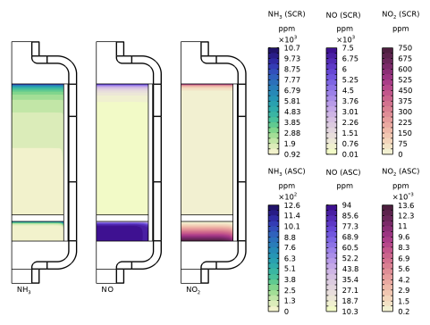
In the tree, select Study 5: Monolith Reactor Model/Solution 23 (12) (sol23) > Transport of Diluted Species in Porous Media > Plot array: Concentrations, H2O, NH3, NO, NO2 (tds).
4
Click the Add Result Template button in the window toolbar.
Results
Nitrogen Species Molar Fractions
1
In the Settings window for 2D Plot Group, type Nitrogen Species Molar Fractions in the Label text field.
2
Locate the Data section. From the Dataset list, choose Study 5: Monolith Reactor Model/Parametric Solutions 5 (16) (sol25).
3
From the Cases list, choose Low Load.
4
Click to expand the Title section. From the Title type list, choose None.
5
Click to expand the Plot Array section. In the Relative padding text field, type 0.3.
6
In the Model Builder window, expand the Nitrogen Species Molar Fractions node.
H2O, Surface, H2O, Total Flux, H2O, Total Flux, NH3, Total Flux, NO, Total Flux, NO2
1
In the Model Builder window, under Results > Nitrogen Species Molar Fractions, Ctrl-click to select Surface, H2O, Total Flux, H2O, H2O, Total Flux, NH3, Total Flux, NO, and Total Flux, NO2.
2
Surface, NH3 (SCR)
1
In the Settings window for Surface, type Surface, NH3 (SCR) in the Label text field.
2
Locate the Expression section. In the Expression text field, type yNH3.
3
From the Unit list, choose ppm.
4
Locate the Coloring and Style section. From the Color table list, choose Cynanthus.
5
In the Color legend title text field, type NH<sub>3</sub> (SCR).
6
From the Color table type list, choose Discrete.
7
In the Number of bands text field, type 20.
Selection 1
1
Right-click Surface, NH3 (SCR) and choose Selection.
2
Click the  Zoom Extents button in the Graphics toolbar.
3
Surface, NH3 (ASC)
1
Right-click Surface, NH3 (SCR) and choose Duplicate.
2
In the Settings window for Surface, type Surface, NH3 (ASC) in the Label text field.
3
Locate the Coloring and Style section. In the Color legend title text field, type NH<sub>3</sub> (ASC).
Selection 1
1
In the Model Builder window, expand the Surface, NH3 (ASC) node, then click Selection 1.
2
In the Settings window for Selection, locate the Selection section.
3
Click to select the  Activate Selection toggle button.
4
Surface, NO (SCR)
1
In the Model Builder window, under Results > Nitrogen Species Molar Fractions click Surface, NO.
2
In the Settings window for Surface, locate the Expression section.
3
In the Expression text field, type yNO.
4
From the Unit list, choose ppm.
5
Locate the Coloring and Style section. From the Color table list, choose Baptisia.
6
In the Color legend title text field, type NO (SCR).
7
From the Color table type list, choose Discrete.
8
In the Number of bands text field, type 20.
9
In the Label text field, type Surface, NO (SCR).
Selection 1
1
Right-click Surface, NO (SCR) and choose Selection.
2
Surface, NO (ASC)
1
Right-click Surface, NO (SCR) and choose Duplicate.
2
In the Settings window for Surface, type Surface, NO (ASC) in the Label text field.
3
Locate the Coloring and Style section. In the Color legend title text field, type NO (ASC).
Selection 1
1
In the Model Builder window, expand the Surface, NO (ASC) node, then click Selection 1.
2
In the Settings window for Selection, locate the Selection section.
3
Click to select the  Activate Selection toggle button.
4
Surface, NO2 (SCR)
1
In the Model Builder window, under Results > Nitrogen Species Molar Fractions click Surface, NO2.
2
In the Settings window for Surface, type Surface, NO2 (SCR) in the Label text field.
3
Locate the Expression section. In the Expression text field, type yNO2.
4
From the Unit list, choose ppm.
5
Locate the Coloring and Style section. From the Color table list, choose Arctium.
6
In the Color legend title text field, type NO<sub>2</sub> (SCR).
7
From the Color table type list, choose Discrete.
8
In the Number of bands text field, type 20.
Selection 1
1
Right-click Surface, NO2 (SCR) and choose Selection.
2
Surface, NO2 (ASC)
1
Right-click Surface, NO2 (SCR) and choose Duplicate.
2
In the Settings window for Surface, type Surface, NO2 (ASC) in the Label text field.
3
Locate the Coloring and Style section. In the Color legend title text field, type NO<sub>2</sub> (ASC).
Surface, NH3 (ASC)
1
In the Model Builder window, expand the Surface, NO2 (ASC) node, then click Surface, NH3 (ASC).
2
Surface, NO (ASC)
1
In the Model Builder window, click Surface, NO (ASC).
2
Nitrogen Species Molar Fractions
Optionally, edit the plot array indices to start from zero instead of from one.
Surface, NH3 (SCR)
1
In the Model Builder window, expand the Results > Nitrogen Species Molar Fractions node, then click Surface, NH3 (SCR).
2
In the Settings window for Surface, click to expand the Plot Array section.
3
In the Index text field, type 0.
Surface, NH3 (ASC)
1
In the Model Builder window, click Surface, NH3 (ASC).
2
In the Settings window for Surface, locate the Plot Array section.
3
In the Index text field, type 0.
Surface, NO (SCR)
1
In the Model Builder window, click Surface, NO (SCR).
2
In the Settings window for Surface, locate the Plot Array section.
3
In the Index text field, type 1.
Surface, NO (ASC)
1
In the Model Builder window, click Surface, NO (ASC).
2
In the Settings window for Surface, locate the Plot Array section.
3
In the Index text field, type 1.
Surface, NO2 (SCR)
1
In the Model Builder window, click Surface, NO2 (SCR).
2
In the Settings window for Surface, locate the Plot Array section.
3
In the Index text field, type 2.
Surface, NO2 (ASC)
1
In the Model Builder window, click Surface, NO2 (ASC).
2
In the Settings window for Surface, locate the Plot Array section.
3
In the Index text field, type 2.
NH3
1
In the Model Builder window, click NH3.
2
In the Settings window for Annotation, locate the Annotation section.
3
In the Text text field, type NH$_3$.
4
Select the LaTeX markup checkbox.
5
Click to expand the Plot Array section. In the Index text field, type 0.
NO
1
In the Model Builder window, click NO.
2
In the Settings window for Annotation, locate the Plot Array section.
3
In the Index text field, type 1.
NO2
1
In the Model Builder window, click NO2.
2
In the Settings window for Annotation, locate the Annotation section.
3
In the Text text field, type NO$_2$.
4
Select the LaTeX markup checkbox.
5
Locate the Plot Array section. In the Index text field, type 2.
Selection 1
1
In the Model Builder window, under Results > Nitrogen Species Molar Fractions > Surface, NO2 (ASC) click Selection 1.
2
In the Settings window for Selection, locate the Selection section.
3
Click to select the  Activate Selection toggle button.
4
5
Click the  Zoom Extents button in the Graphics toolbar.
6
In the Nitrogen Species Molar Fractions toolbar, click  Plot.
7
Click the  Show Grid button in the Graphics toolbar.
Nitrogen Species Molar Fractions
Switch between the cases to see the different results.
1
In the Model Builder window, under Results click Nitrogen Species Molar Fractions.
2
In the Settings window for 2D Plot Group, locate the Data section.
3
From the Cases list, choose Intermediate Load.
4
Click the  Zoom Extents button in the Graphics toolbar.
5
In the Nitrogen Species Molar Fractions toolbar, click  Plot.
6
From the Cases list, choose High Load.
7
Click the  Zoom Extents button in the Graphics toolbar.
8
In the Nitrogen Species Molar Fractions toolbar, click  Plot.
The following steps generate Figure 6.
Drive Cases, ANR = 1.3, T, U, and dP
1
In the Results toolbar, click  2D Plot Group.
2
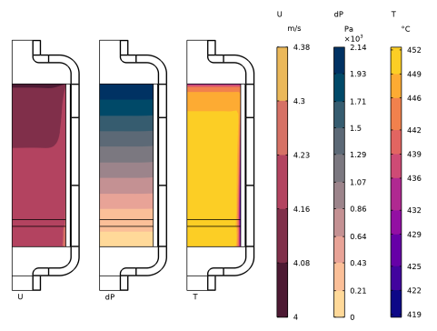
In the Settings window for 2D Plot Group, type Drive Cases, ANR = 1.3, T, U, and dP in the Label text field.
3
Locate the Data section. From the Dataset list, choose Study 5: Monolith Reactor Model/Parametric Solutions 5 (16) (sol25).
4
Locate the Title section. From the Title type list, choose None.
5
Locate the Color Legend section. Select the Show titles checkbox.
6
Select the Show units checkbox.
7
Click to expand the Plot Array section. From the Array type list, choose Linear.
Surface 1
In the Results toolbar, click  More Datasets and choose Surface.
Drive Cases, ANR = 1.3, T, U, and dP
In the Model Builder window, under Results click Drive Cases, ANR = 1.3, T, U, and dP.
Velocity
1
In the Drive Cases, ANR = 1.3, T, U, and dP toolbar, click  Surface.
2
In the Settings window for Surface, type Velocity in the Label text field.
3
Locate the Expression section. In the Expression text field, type spf.U.
4
Locate the Coloring and Style section. From the Color table list, choose Metasepia.
5
In the Color legend title text field, type U.
6
From the Color table transformation list, choose Reverse.
7
From the Color table type list, choose Discrete.
8
In the Number of bands text field, type 5.
Drive Cases, ANR = 1.3, T, U, and dP
In the Drive Cases, ANR = 1.3, T, U, and dP toolbar, click  Annotation.
U
1
In the Settings window for Annotation, type U in the Label text field.
2
Locate the Annotation section. In the Text text field, type U.
3
Locate the Position section. In the z text field, type -0.21.
4
Locate the Coloring and Style section. Clear the Show point checkbox.
5
Click to expand the Plot Array section. Select the Manual indexing checkbox.
Drive Cases, ANR = 1.3, T, U, and dP
In the Drive Cases, ANR = 1.3, T, U, and dP toolbar, click  Surface.
Pressure
1
In the Settings window for Surface, type Pressure in the Label text field.
2
Locate the Expression section. In the Expression text field, type p.
3
Locate the Coloring and Style section. From the Color table list, choose Agama.
4
In the Color legend title text field, type dP.
5
From the Color table type list, choose Discrete.
Drive Cases, ANR = 1.3, T, U, and dP
In the Drive Cases, ANR = 1.3, T, U, and dP toolbar, click  Annotation.
dP
1
In the Settings window for Annotation, type dP in the Label text field.
2
Locate the Annotation section. In the Text text field, type dP.
3
Locate the Position section. In the z text field, type -0.21.
4
Locate the Coloring and Style section. Clear the Show point checkbox.
5
Locate the Plot Array section. Select the Manual indexing checkbox.
6
In the Index text field, type 1.
Drive Cases, ANR = 1.3, T, U, and dP
In the Drive Cases, ANR = 1.3, T, U, and dP toolbar, click  Surface.
Temperature
1
In the Settings window for Surface, type Temperature in the Label text field.
2
Locate the Expression section. In the Expression text field, type T.
3
From the Unit list, choose °C.
4
Locate the Coloring and Style section. From the Color table list, choose Plasma.
5
In the Color legend title text field, type T.
6
From the Color table type list, choose Discrete.
Selection 1
1
In the Drive Cases, ANR = 1.3, T, U, and dP toolbar, click  Selection.
2
In the Settings window for Selection, locate the Selection section.
3
From the Selection list, choose Porous and Free Flow Domains.
Drive Cases, ANR = 1.3, T, U, and dP
In the Drive Cases, ANR = 1.3, T, U, and dP toolbar, click  Annotation.
T
1
In the Settings window for Annotation, type T in the Label text field.
2
Locate the Annotation section. In the Text text field, type T.
3
Locate the Position section. In the z text field, type -0.21.
4
Locate the Coloring and Style section. Clear the Show point checkbox.
5
Locate the Plot Array section. Select the Manual indexing checkbox.
6
In the Index text field, type 2.
7
Click the  Zoom Extents button in the Graphics toolbar.
8
In the Drive Cases, ANR = 1.3, T, U, and dP toolbar, click  Plot.
The following steps generate Figure 7.
Conversions, NH3 and NOx
1
In the Results toolbar, click  1D Plot Group.
2
In the Settings window for 1D Plot Group, type Conversions, NH3 and NOx in the Label text field.
3
Locate the Data section. From the Dataset list, choose Study 5: Monolith Reactor Model/Parametric Solutions 5 (16) (sol25).
4
Click to expand the Title section. From the Title type list, choose None.
5
Locate the Plot Settings section.
6
Select the y-axis label checkbox. In the associated text field, type Conversion.
NH3 center
1
In the Conversions, NH3 and NOx toolbar, click  Line Graph.
2
In the Settings window for Line Graph, type NH3 center in the Label text field.
3
4
Locate the y-Axis Data section. In the Expression text field, type X_NH3.
5
Select the Description checkbox. In the associated text field, type Conversion.
6
Locate the x-Axis Data section. From the Parameter list, choose Expression.
7
In the Expression text field, type (0.4-z)*pi*d_cat^2/4.
8
Select the Description checkbox. In the associated text field, type Volume.
9
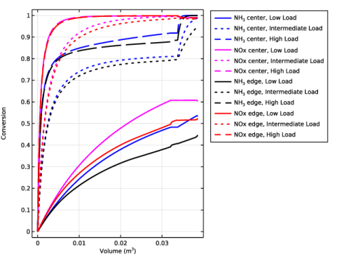
Click to expand the Coloring and Style section. Find the Line style subsection. From the Line list, choose Cycle.
10
From the Color list, choose Blue.
11
From the Width list, choose 2.
12
Click to expand the Legends section. Select the Show legends checkbox.
13
Find the Prefix and suffix subsection. In the Prefix text field, type NH<sub>3</sub> center, .
NOx center
1
Right-click NH3 center and choose Duplicate.
2
In the Settings window for Line Graph, type NOx center in the Label text field.
3
4
Locate the y-Axis Data section. In the Expression text field, type X_NOx.
5
Locate the Coloring and Style section. Find the Line style subsection. From the Line list, choose Cycle (reset).
6
From the Color list, choose Magenta.
7
Locate the Legends section. Find the Prefix and suffix subsection. In the Prefix text field, type NOx center, .
NH3 center, NOx center
1
In the Model Builder window, under Results > Conversions, NH3 and NOx, Ctrl-click to select NH3 center and NOx center.
2
NH3 edge
1
In the Settings window for Line Graph, type NH3 edge in the Label text field.
2
Locate the Selection section. Click  Clear Selection.
3
4
Locate the Coloring and Style section. Find the Line style subsection. From the Line list, choose Cycle (reset).
5
From the Color list, choose Black.
6
Locate the Legends section. Find the Prefix and suffix subsection. In the Prefix text field, type NH<sub>3</sub> edge, .
NOx edge
1
In the Model Builder window, under Results > Conversions, NH3 and NOx click NOx center 1.
2
In the Settings window for Line Graph, type NOx edge in the Label text field.
3
Locate the Selection section. Click  Clear Selection.
4
5
Locate the Coloring and Style section. From the Color list, choose Red.
6
Locate the Legends section. Find the Prefix and suffix subsection. In the Prefix text field, type NOx edge, .
Conversions, NH3 and NOx
1
In the Model Builder window, click Conversions, NH3 and NOx.
2
In the Settings window for 1D Plot Group, click to expand the Window Settings section.
3
Locate the Legend section. From the Layout list, choose Outside graph axis area.
4
Click the  Zoom Extents button in the Graphics toolbar.
5
In the Conversions, NH3 and NOx toolbar, click  Plot.
The following steps generate Figure 8.
Temperature Difference Along Reactor Axis
1
In the Home toolbar, click  Add Plot Group and choose 1D Plot Group.
2
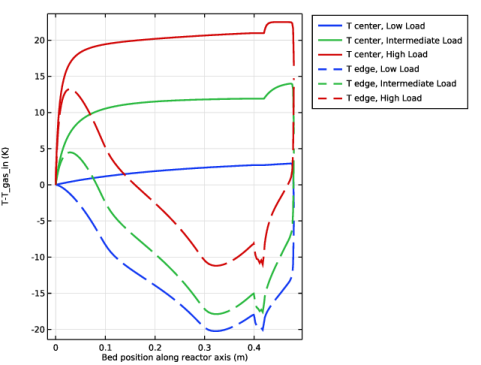
In the Settings window for 1D Plot Group, type Temperature Difference Along Reactor Axis in the Label text field.
3
Locate the Data section. From the Dataset list, choose Study 5: Monolith Reactor Model/Parametric Solutions 5 (16) (sol25).
4
Locate the Title section. From the Title type list, choose None.
5
Locate the Plot Settings section.
6
Select the x-axis label checkbox. In the associated text field, type Bed position along reactor axis (m).
7
Locate the Legend section. From the Layout list, choose Outside graph axis area.
Temperature At Reactor Center
1
Right-click Temperature Difference Along Reactor Axis and choose Line Graph.
2
In the Settings window for Line Graph, type Temperature At Reactor Center in the Label text field.
3
4
Locate the y-Axis Data section. In the Expression text field, type T-T_gas_in.
5
Locate the x-Axis Data section. From the Parameter list, choose Reversed arc length.
6
Locate the Coloring and Style section. From the Width list, choose 2.
7
Locate the Legends section. Select the Show legends checkbox.
8
Find the Prefix and suffix subsection. In the Prefix text field, type T center, .
Temperature At Bed Edge
1
Right-click Temperature At Reactor Center and choose Duplicate.
2
In the Settings window for Line Graph, type Temperature At Bed Edge in the Label text field.
3
Locate the Selection section. Click  Clear Selection.
4
5
Locate the Coloring and Style section. Find the Line style subsection. From the Line list, choose Dashed.
6
From the Color list, choose Cycle (reset).
7
From the Width list, choose 2.
8
Locate the Legends section. Find the Prefix and suffix subsection. In the Prefix text field, type T edge, .
9
Click the  Zoom Extents button in the Graphics toolbar.
10
In the Temperature Difference Along Reactor Axis toolbar, click  Plot.
As a final evaluation, derive the average molar fraction of NH3 and NOx out from the first bed, as well as out from the reactor.
Line Average SCR Outlet
1
In the Results toolbar, click  More Derived Values and choose Average > Line Average.
2
In the Settings window for Line Average, type Line Average SCR Outlet in the Label text field.
3
Locate the Data section. From the Dataset list, choose Study 5: Monolith Reactor Model/Parametric Solutions 5 (16) (sol25).
4
5
Locate the Expressions section. In the table, enter the following settings:
6
Clicknext to  Evaluate, then choose New Table.
Line Average Reactor Outlet
1
Right-click Line Average SCR Outlet and choose Duplicate.
2
In the Settings window for Line Average, type Line Average Reactor Outlet in the Label text field.
3
4
Clicknext to  Evaluate, then choose New Table.
The following steps generate the thumbnail for this model.
Concentration and Temperature Profiles
1
In the Results toolbar, click  3D Plot Group.
2
In the Settings window for 3D Plot Group, type Concentration and Temperature Profiles in the Label text field.
Revolution 2D 1
1
In the Results toolbar, click  More Datasets and choose Revolution 2D.
2
In the Settings window for Revolution 2D, locate the Data section.
3
From the Dataset list, choose Study 5: Monolith Reactor Model/Parametric Solutions 5 (16) (sol25).
4
Click to expand the Revolution Layers section. In the Start angle text field, type -90.
5
In the Revolution angle text field, type 200.
Concentration and Temperature Profiles
1
In the Model Builder window, under Results click Concentration and Temperature Profiles.
2
In the Settings window for 3D Plot Group, locate the Data section.
3
From the Dataset list, choose Revolution 2D 1.
4
From the Cases list, choose Low Load.
5
Click to expand the Title section. From the Title type list, choose None.
6
Locate the Plot Settings section. From the View list, choose View 3D 4.
7
Clear the Plot dataset edges checkbox.
8
Locate the Color Legend section. Clear the Show legends checkbox.
Surface 1
1
In the Concentration and Temperature Profiles toolbar, click  Surface.
2
In the Settings window for Surface, locate the Expression section.
3
In the Expression text field, type 1.
Selection 1
1
In the Concentration and Temperature Profiles toolbar, click  Selection.
2
In the Settings window for Selection, locate the Selection section.
3
From the Selection list, choose Metal Shell Domain.
Surface 1
In the Model Builder window, click Surface 1.
Material Appearance 1
1
In the Concentration and Temperature Profiles toolbar, click  Material Appearance.
2
In the Settings window for Material Appearance, locate the Appearance section.
3
From the Appearance list, choose Custom.
4
From the Material type list, choose Tungsten.
Concentration and Temperature Profiles
In the Concentration and Temperature Profiles toolbar, click  Surface.
Surface 2
1
In the Settings window for Surface, locate the Expression section.
2
In the Expression text field, type T.
3
Locate the Coloring and Style section. From the Color table list, choose HeatCameraLight.
Selection 1
1
In the Concentration and Temperature Profiles toolbar, click  Selection.
2
In the Settings window for Selection, locate the Selection section.
3
From the Selection list, choose Insulating Gas.
Surface 2
In the Model Builder window, click Surface 2.
Material Appearance 1
1
In the Concentration and Temperature Profiles toolbar, click  Material Appearance.
2
In the Settings window for Material Appearance, locate the Appearance section.
3
From the Material list, choose Air (mat3).
4
Locate the Color section. Select the Use the plot’s color checkbox.
Concentration and Temperature Profiles
In the Concentration and Temperature Profiles toolbar, click  Surface.
Surface 3
1
In the Settings window for Surface, locate the Expression section.
2
In the Expression text field, type T.
3
Locate the Coloring and Style section. From the Color table list, choose HeatCameraLight.
Selection 1
1
In the Concentration and Temperature Profiles toolbar, click  Selection.
2
In the Settings window for Selection, locate the Selection section.
3
From the Selection list, choose Mat Domain.
Surface 3
In the Model Builder window, click Surface 3.
Material Appearance 1
1
In the Concentration and Temperature Profiles toolbar, click  Material Appearance.
2
In the Settings window for Material Appearance, locate the Appearance section.
3
From the Appearance list, choose Custom.
4
From the Material type list, choose Rock.
5
Locate the Color section. Select the Use the plot’s color checkbox.
Concentration and Temperature Profiles
In the Concentration and Temperature Profiles toolbar, click  Surface.
Surface 4
1
In the Settings window for Surface, locate the Expression section.
2
In the Expression text field, type cNO+cNO2.
3
Locate the Coloring and Style section. From the Color table list, choose Cerinthe.
Selection 1
1
In the Concentration and Temperature Profiles toolbar, click  Selection.
2
3
In the Settings window for Selection, locate the Revolution Selection section.
4
Clear the Evaluate the end cap checkbox.
Surface 4
In the Model Builder window, click Surface 4.
Material Appearance 1
1
In the Concentration and Temperature Profiles toolbar, click  Material Appearance.
2
In the Settings window for Material Appearance, locate the Appearance section.
3
From the Appearance list, choose Custom.
4
From the Material type list, choose Rock.
5
Locate the Color section. Select the Use the plot’s color checkbox.
Contour 1
1
In the Model Builder window, right-click Concentration and Temperature Profiles and choose Contour.
2
In the Settings window for Contour, locate the Expression section.
3
In the Expression text field, type cNO+cNO2.
4
Locate the Levels section. In the Total levels text field, type 15.
5
Locate the Coloring and Style section. From the Color table list, choose Prionace.
6
From the Color table transformation list, choose Reverse.
Selection 1
1
In the Concentration and Temperature Profiles toolbar, click  Selection.
2
3
In the Settings window for Selection, locate the Revolution Selection section.
4
Clear the Evaluate the mantle checkbox.
Concentration and Temperature Profiles
In the Concentration and Temperature Profiles toolbar, click  Surface.
Surface 5
1
In the Settings window for Surface, locate the Expression section.
2
In the Expression text field, type 1.
Selection 1
1
In the Concentration and Temperature Profiles toolbar, click  Selection.
2
3
In the Settings window for Selection, locate the Revolution Selection section.
4
Clear the Evaluate the end cap checkbox.
5
Clear the Evaluate the start cap checkbox.
Surface 5
In the Model Builder window, click Surface 5.
Material Appearance 1
1
In the Concentration and Temperature Profiles toolbar, click  Material Appearance.
2
In the Settings window for Material Appearance, locate the Appearance section.
3
From the Appearance list, choose Custom.
4
From the Material type list, choose Custom.
5
Click Define custom colors.
6
7
Click Add to custom colors.
8
Click Show color palette only or OK on the cross-platform desktop.
9
From the Diffuse color list, choose Custom.
10
Click Define custom colors.
11
12
Click Add to custom colors.
13
Click Show color palette only or OK on the cross-platform desktop.
14
From the Edit menu, choose Undo Material Appearance 1: Custom Color.
15
From the Ambient color list, choose Custom.
16
Click Define custom colors.
17
18
Click Add to custom colors.
19
Click Show color palette only or OK on the cross-platform desktop.
20
Select the Custom basis for brush lines checkbox.
21
In the Scale text field, type 2.
22
In the Origin text field, type 1.
23
Select the Specify ym-axis checkbox.
24
Select the Normal mapping checkbox.
25
From the Noise type list, choose Simplex noise.
26
In the Normal vector noise scale text field, type 50.
27
In the Normal vector noise frequency text field, type 50.
28
From the Brush lines list, choose Brush lines orthogonal to xm-axis.
29
In the Surface roughness text field, type 1.
30
In the Diffuse wrap text field, type 0.
31
In the Reflectance text field, type 0.05.
Surface 6
1
Right-click Surface 5 and choose Duplicate.
2
In the Settings window for Surface, locate the Expression section.
3
In the Expression text field, type cNH3.
Selection 1
1
In the Model Builder window, expand the Surface 6 node, then click Selection 1.
2
In the Settings window for Selection, locate the Revolution Selection section.
3
Clear the Evaluate the mantle checkbox.
4
Select the Evaluate the end cap checkbox.
Material Appearance 1
1
In the Model Builder window, click Material Appearance 1.
2
In the Settings window for Material Appearance, locate the Color section.
3
Select the Use the plot’s color checkbox.
Surface 6
1
In the Model Builder window, click Surface 6.
2
In the Settings window for Surface, locate the Coloring and Style section.
3
From the Color table list, choose Kyanite.
4
In the Concentration and Temperature Profiles toolbar, click  Plot.
Add the result plots from Study 5 in a group.
Concentration and Temperature Profiles, Conversions, NH3 and NOx, Drive Cases, ANR = 1.3, T, U, and dP, Nitrogen Species Molar Fractions, Temperature Difference Along Reactor Axis
1
In the Model Builder window, under Results, Ctrl-click to select Nitrogen Species Molar Fractions, Drive Cases, ANR = 1.3, T, U, and dP, Conversions, NH3 and NOx, Temperature Difference Along Reactor Axis, and Concentration and Temperature Profiles.
2
Monolith Reactor Model
In the Settings window for Group, type Monolith Reactor Model in the Label text field.
Appendix — Geometry Modeling Instructions
From the File menu, choose New.
New
In the New window, click  Blank Model.
Global Definitions
Parameters 1
1
In the Model Builder window, under Global Definitions click Parameters 1.
2
In the Settings window for Parameters, locate the Parameters section.
3
Click  Load from File.
4
Add Component
In the Home toolbar, click  Add Component and choose 2D Axisymmetric.
Geometry 1
SCR (selective catalytic reduction) monolith
1
In the Geometry toolbar, click  Rectangle.
2
In the Settings window for Rectangle, type SCR (selective catalytic reduction) monolith in the Label text field.
3
Locate the Size and Shape section. In the Width text field, type d_cat/2.
4
In the Height text field, type l_SCR.
5
Click to expand the Layers section.
Mat
1
In the Geometry toolbar, click  Rectangle.
2
In the Settings window for Rectangle, type Mat in the Label text field.
3
Locate the Size and Shape section. In the Width text field, type matThickness+shellThickness.
4
In the Height text field, type l_SCR+freeFlowHeight+l_ASC.
5
Locate the Position section. In the r text field, type d_cat/2.
6
In the z text field, type -freeFlowHeight-l_ASC.
7
Locate the Layers section. In the table, enter the following settings:
8
Select the Layers to the right checkbox.
9
Clear the Layers on bottom checkbox.
Free Flow
1
In the Geometry toolbar, click  Rectangle.
2
In the Settings window for Rectangle, type Free Flow in the Label text field.
3
Locate the Size and Shape section. In the Width text field, type d_cat/2+shellThickness-shellThickness.
4
In the Height text field, type freeFlowHeight.
5
Locate the Position section. In the z text field, type -0.02.
ASC (ammonia slip catalyst)
1
Right-click Free Flow and choose Duplicate.
2
In the Settings window for Rectangle, type ASC (ammonia slip catalyst) in the Label text field.
3
Locate the Size and Shape section. In the Width text field, type d_cat/2.
4
In the Height text field, type l_ASC.
5
Locate the Position section. In the z text field, type -freeFlowHeight-l_ASC.
Thicken 1 (thi1)
1
In the Geometry toolbar, click  Conversions and choose Thicken.
2
In the Settings window for Thicken, locate the Input section.
3
From the Geometric entity level list, choose Boundary.
4
On the object r2, select Boundary 7 only.
5
Select the Keep input objects checkbox.
6
Locate the Options section. From the Offset list, choose Asymmetric.
7
In the Upside thickness text field, type shellThickness.
8
From the Convex corner handling list, choose Tangent lines.
Union 1 (uni1)
1
In the Geometry toolbar, click  Booleans and Partitions and choose Union.
2
3
In the Settings window for Union, locate the Union section.
4
Click the  Remove from Selection button for Input objects.
5
Clear the Keep interior boundaries checkbox.
Gas Box
1
In the Geometry toolbar, click  Rectangle.
2
In the Settings window for Rectangle, type Gas Box in the Label text field.
3
Locate the Size and Shape section. In the Width text field, type boxThickness.
4
In the Height text field, type l_ASC+freeFlowHeight+l_SCR.
5
Locate the Position section. In the r text field, type d_cat/2+matThickness+shellThickness+shellThickness.
6
In the z text field, type -l_ASC-freeFlowHeight.
7
Locate the Layers section. In the table, enter the following settings:
8
Select the Layers to the right checkbox.
9
Select the Layers on top checkbox.
Inlet
1
In the Geometry toolbar, click  Rectangle.
2
In the Settings window for Rectangle, type Inlet in the Label text field.
3
Locate the Size and Shape section. In the Width text field, type inletInnerD.
4
In the Height text field, type inletHeight.
5
Locate the Position section. In the z text field, type l_SCR+inletHeight*2.
Inlet Box
1
In the Geometry toolbar, click  Rectangle.
2
In the Settings window for Rectangle, type Inlet Box in the Label text field.
3
Locate the Size and Shape section. In the Width text field, type boxThickness.
4
In the Height text field, type inletHeight.
5
Locate the Position section. In the r text field, type inletInnerD.
6
In the z text field, type l_SCR+inletHeight*2.
7
Locate the Layers section. In the table, enter the following settings:
8
Select the Layers to the left checkbox.
9
Select the Layers to the right checkbox.
10
Select the Layers on top checkbox.
Help Rectangle Top
1
In the Geometry toolbar, click  Rectangle.
2
In the Settings window for Rectangle, type Help Rectangle Top in the Label text field.
3
Locate the Size and Shape section. In the Width text field, type totalWidth-inletInnerD.
4
In the Height text field, type inletHeight*2.
5
Locate the Position section. In the r text field, type inletInnerD.
6
In the z text field, type l_SCR.
7
Locate the Layers section. In the table, enter the following settings:
8
Select the Layers to the left checkbox.
9
Select the Layers to the right checkbox.
10
Clear the Layers on bottom checkbox.
11
Select the Layers on top checkbox.
Help Rectangle Horizontal Small Top
1
In the Geometry toolbar, click  Rectangle.
2
In the Settings window for Rectangle, type Help Rectangle Horizontal Small Top in the Label text field.
3
Locate the Size and Shape section. In the Width text field, type totalWidth - inletInnerD.
4
In the Height text field, type boxThickness.
5
Locate the Position section. In the r text field, type inletInnerD.
6
In the z text field, type l_SCR+inletHeight*2-boxThickness.
7
Locate the Layers section. In the table, enter the following settings:
Help Rectangle Vertical Top
1
In the Geometry toolbar, click  Rectangle.
2
In the Settings window for Rectangle, type Help Rectangle Vertical Top in the Label text field.
3
Locate the Size and Shape section. In the Width text field, type boxThickness+shellThickness.
4
In the Height text field, type inletHeight*2.
5
Locate the Position section. In the r text field, type d_cat/2+matThickness+shellThickness.
6
In the z text field, type l_SCR.
7
Locate the Layers section. In the table, enter the following settings:
8
Select the Layers to the left checkbox.
9
Select the Layers to the right checkbox.
10
Clear the Layers on bottom checkbox.
Quadratic Bézier 1 (qb1)
1
In the Geometry toolbar, click  More Primitives and choose Quadratic Bézier.
2
In the Settings window for Quadratic Bézier, locate the Control Points section.
3
In row 1, set r to 0.14.
4
In row 1, set z to 0.462.
5
In row 2, set r to 0.174651.
6
In row 2, set z to 0.462.
7
In row 3, set r to 0.1746619234313964.
8
In row 3, set z to 0.4301309883594513.
Quadratic Bézier 2 (qb2)
1
In the Geometry toolbar, click  More Primitives and choose Quadratic Bézier.
2
In the Settings window for Quadratic Bézier, locate the Control Points section.
3
In row 1, set r to 0.14.
4
In row 1, set z to 0.463651.
5
In row 2, set r to 0.176302.
6
In row 2, set z to 0.463651.
7
In row 3, set r to 0.17631292343140004.
8
In row 3, set z to 0.4301309883594513.
Quadratic Bézier 3 (qb3)
1
In the Geometry toolbar, click  More Primitives and choose Quadratic Bézier.
2
In the Settings window for Quadratic Bézier, locate the Control Points section.
3
In row 1, set r to 0.14.
4
In row 1, set z to 0.484349.
5
In row 2, set r to 0.198651.
6
In row 2, set z to 0.48448984122275995.
7
In row 3, set r to 0.198651.
8
In row 3, set z to 0.4301309883594513.
Quadratic Bézier 4 (qb4)
1
In the Geometry toolbar, click  More Primitives and choose Quadratic Bézier.
2
In the Settings window for Quadratic Bézier, locate the Control Points section.
3
In row 1, set r to 0.14.
4
In row 1, set z to 0.486.
5
In row 2, set r to 0.200302.
6
In row 2, set z to 0.48614084122275997.
7
In row 3, set r to 0.200302.
8
In row 3, set z to 0.4301309883594513.
Quadratic Bézier 5 (qb5)
1
In the Geometry toolbar, click  More Primitives and choose Quadratic Bézier.
2
In the Settings window for Quadratic Bézier, locate the Control Points section.
3
In row 1, set r to 0.062738.
4
In row 1, set z to 0.48.
5
In row 2, set r to 0.062738.
6
In row 2, set z to 0.463651.
7
In row 3, set r to 0.08.
8
In row 3, set z to 0.463651.
Quadratic Bézier 6 (qb6)
1
In the Geometry toolbar, click  More Primitives and choose Quadratic Bézier.
2
In the Settings window for Quadratic Bézier, locate the Control Points section.
3
In row 1, set r to 0.061087.
4
In row 1, set z to 0.48.
5
In row 2, set r to 0.061087.
6
In row 2, set z to 0.462.
7
In row 3, set r to 0.08.
8
In row 3, set z to 0.462.
Mirror 1 (mir1)
1
In the Geometry toolbar, click  Transforms and choose Mirror.
2
In the Settings window for Mirror, locate the Input section.
3
Select the Keep input objects checkbox.
4
Click the  Zoom Extents button in the Graphics toolbar.
5
In the Graphics window toolbar, clicknext to  Select Objects, then choose Select Objects.
6
Select the objects qb1, qb2, qb3, qb4, qb5, qb6, r10, r6, r7, r8, and r9 only.
7
8
Locate the Line of Reflection section. From the Specify list, choose Edge.
9
On the object r8, select Boundary 7 only.
10
Locate the Selections of Resulting Entities section. Select the Resulting objects selection checkbox.
Move 1 (mov1)
1
In the Geometry toolbar, click  Transforms and choose Move.
2
In the Settings window for Move, locate the Input section.
3
From the Input objects list, choose Mirror 1.
4
Locate the Displacement section. From the Specify list, choose Positions.
5
Click to select the  Activate Selection toggle button for Vertex to move.
6
On the object mir1(10), select Point 10 only.
7
Click to select the  Activate Selection toggle button for Vertices to move to.
8
On the object r5, select Point 9 only.
Rectangle 11 (r11)
1
In the Geometry toolbar, click  Rectangle.
2
In the Settings window for Rectangle, locate the Size and Shape section.
3
In the Width text field, type totalWidth.
4
In the Height text field, type l_SCR+inletHeight*2+freeFlowHeight+l_ASC+inletHeight*2.
5
Locate the Position section. In the z text field, type -freeFlowHeight-l_ASC-inletHeight*2.
Shell Support Top
1
In the Geometry toolbar, click  Rectangle.
2
In the Settings window for Rectangle, type Shell Support Top in the Label text field.
3
Locate the Size and Shape section. In the Width text field, type shellThickness.
4
In the Height text field, type boxThickness.
5
Locate the Position section. In the r text field, type 0.108.
6
In the z text field, type 0.462.
Shell Support Bottom
1
Right-click Shell Support Top and choose Duplicate.
2
In the Settings window for Rectangle, type Shell Support Bottom in the Label text field.
3
Locate the Position section. In the z text field, type -0.166.
Shell Support Side Top
1
In the Geometry toolbar, click  Rectangle.
2
In the Settings window for Rectangle, type Shell Support Side Top in the Label text field.
3
Locate the Size and Shape section. In the Width text field, type boxThickness.
4
In the Height text field, type shellThickness.
5
Locate the Position section. In the r text field, type 0.1763.
6
In the z text field, type 0.3.
Shell Support Side Bottom
1
Right-click Shell Support Side Top and choose Duplicate.
2
In the Settings window for Rectangle, type Shell Support Side Bottom in the Label text field.
3
Locate the Position section. In the r text field, type 0.17465.
4
In the z text field, type 0.1.
Partition Edges 1 (pare1)
1
In the Geometry toolbar, click  Booleans and Partitions and choose Partition Edges.
2
On the object r5, select Boundary 10 only.
3
In the Settings window for Partition Edges, locate the Positions section.
4
From the Type of specification list, choose Vertex projection.
5
On the object r15, select Points 2 and 3 only.
Ignore Edges 1 (ige1)
1
In the Geometry toolbar, click  Virtual Operations and choose Ignore Edges.
2
On the object fin, select Boundaries 14, 19, 21, 23, 25–30, 32, 34–37, 40, 42, 44, 46, 48, 53, 54, 58–63, 65, 67–71, 73, 78, 79, 82, 83, 88, 91, 93, 94, 96, 98–100, 110, 113–115, 117, 120–122, 124, 128, 131, 135, 138–141, 143–150, 159–169, 172, 174, 175, 177, 179–191, 194–203, 205, 209, 213, 217, 221–247, 249, 250, 252–254, 256, 257, 259–261, 263–277, 283–286, 313, 314, 320, and 321 only.
SCR Catalyst
1
In the Geometry toolbar, click  Selections and choose Explicit Selection.
2
In the Settings window for Explicit Selection, type SCR Catalyst in the Label text field.
3
Click the  Zoom Box button in the Graphics toolbar.
4
On the object ige1, select Domain 5 only.
ASC Catalyst
1
In the Geometry toolbar, click  Selections and choose Explicit Selection.
2
In the Settings window for Explicit Selection, type ASC Catalyst in the Label text field.
3
On the object ige1, select Domain 3 only.
Mat Domain
1
In the Geometry toolbar, click  Selections and choose Explicit Selection.
2
In the Settings window for Explicit Selection, type Mat Domain in the Label text field.
3
On the object ige1, select Domain 14 only.
Metal Shell Domain
1
In the Geometry toolbar, click  Selections and choose Explicit Selection.
2
In the Settings window for Explicit Selection, type Metal Shell Domain in the Label text field.
3
On the object ige1, select Domains 7 and 15 only.
Flow Inlet
1
In the Geometry toolbar, click  Selections and choose Explicit Selection.
2
In the Settings window for Explicit Selection, type Flow Inlet in the Label text field.
3
Click the  Zoom Extents button in the Graphics toolbar.
4
Locate the Entities to Select section. From the Geometric entity level list, choose Boundary.
5
On the object ige1, select Boundary 12 only.
Flow Outlet
1
In the Geometry toolbar, click  Selections and choose Explicit Selection.
2
In the Settings window for Explicit Selection, type Flow Outlet in the Label text field.
3
Locate the Entities to Select section. From the Geometric entity level list, choose Boundary.
4
On the object ige1, select Boundary 6 only.
Free Flow Domain
1
In the Geometry toolbar, click  Selections and choose Explicit Selection.
2
In the Settings window for Explicit Selection, type Free Flow Domain in the Label text field.
3
On the object ige1, select Domain 4 only.
Insulating Gas
1
In the Geometry toolbar, click  Selections and choose Explicit Selection.
2
In the Settings window for Explicit Selection, type Insulating Gas in the Label text field.
3
Click the  Zoom Box button in the Graphics toolbar.
4
On the object ige1, select Domains 8–13 and 16–18 only.