PDF

Analysis of NOx and Ammonia Conversion Kinetics in a Dual-Bed Plug-Flow Reactor
Introduction
This example looks at the reduction of harmful nitrogen oxides NOx (NO and NO2) into nitrogen in an exhaust gas after-treatment system of a heavy-duty diesel truck. The nitrogen oxides are reduced by ammonia that is injected upstream of the after-treatment system consisting of a catalytic, monolithic reactor.
The reactor has two catalytic beds with two different catalysts. The upstream bed is a selective catalytic reduction (SCR) bed with the purpose of selectively convert NOx to nitrogen. The second bed is an ammonia-slip-catalyst (ASC). This bed should convert the remaining ammonia to nitrogen.
The dosing rate of ammonia has a direct influence on the conversion of NOx. Too low dosing rate leads to exhaust of unconverted nitrogen oxides, while too much ammonia may give ammonia-slip, or even NOx emissions, since a side reaction in the ammonia-slip bed is formation of NOx from ammonia. Since the engine load affects the exhaust gas temperature, the volumetric flow rate of exhaust gas, as well as the concentration of former nitrogen oxide, the dosing needs to be dynamically adjusted.
This tutorial aims at getting a primary understanding of the chemical kinetics in the dual-bed reactor. This is achieved by solving the model with the Plug Flow ideal reactor type in the Reaction Engineering interface. The influence of temperature, volumetric flow rate, and ammonia-to-NOx ratio is investigated.
Model Definition
Chemical Reactions
In this tutorial model, a simplified reaction setup is used with six reactions in the first bed, and four reactions in the second bed.
In the selective catalytic reduction bed, there are three desired SCR reactions that take place. These are the so called standard SCR reaction
(1),
the fast SCR reaction
(2),
and the NO2 SCR reaction
(3).
There is also the oxidation of nitrogen monoxide into nitrogen dioxide
(4).
Finally, there are also two undesired reactions present. It is the oxidation of ammonia into nitrogen
(5),
and the oxidation of ammonia into nitrogen oxide
(6).
Except for the homogeneous gas phase equilibrium reaction (4), all reactions are heterogeneous catalytic reactions with reaction rates that depend on surface coverage. The surface coverage of ammonia can be related to the fluid phase concentration by assuming that ammonia desorption and adsorption are in equilibrium. With a Langmuir-Hinshelwood mechanism, based on this assumption, global rate expressions can be derived. The following five rate expressions have been suggested in Ref. 1:
.
Here, KNH3 is the ammonia adsorption equilibrium constant, expressed with the pre-exponential factor KNH3,523, and the adsorption enthalpy ΔHads:
.
The rate expression for the fast SCR reaction is
.
Correspondingly, the rate expression for the NO2-SCR reaction is
.
The equilibrium rate expression follows the mass action law, giving the forward rate
.
The reversed reaction rate is derived from the forward reaction rate and the equilibrium constant Keq that is derived from thermodynamics laws:
.
The reaction rate expression for the undesired oxidation of ammonia into nitrogen is defined as
.
The reaction rate for the undesired oxidation of ammonia into nitrogen monoxide also follows a Langmuir–Hinshelwood mechanism, and has been suggested to take this form (Ref. 2):
.
Here, G is a variable that accounts for the inhibition effects caused by adsorption of other species on the surface:
,
where Ki (i = 1,…,4) follows an Arrhenius-type expression
.
In the ammonia slip catalyst bed, there is one desired, two undesired reactions, and Reaction 4, the homogeneous equilibrium, that take place. The desired reaction is the oxidation of ammonia to form nitrogen:
(7).
The two undesired reactions are the oxidation of ammonia into nitrogen monoxide
(8),
and the oxidation of ammonia into nitrogen dioxide
(9).
Reactions 7 and 8 are the same chemical equations as Reactions 5 and 6, but since the catalyst is different, the kinetic parameters differ. The rate expressions are assumed the same though. The rate expression for Reaction 9 is
.
The competing chemical reactions raise the issue of optimal dosing of NH3 to handle the reduction process in the first bed. Stoichiometry suggests a 1:1 ratio of NH3 to NO as a lower limit for the standard SCR reaction. Due to the undesired oxidation of ammonia it is likely that a stoichiometric excess of NH3 is necessary. The excess ammonia will be converted in the second ammonia-slip catalyst bed. The NOx forming side reactions in the second bed motivates as low ammonia injection as possible. This is also important for economic and pressure-drop reasons.
SINGLE CHANNEL MODEL
To find the lowest level of NH3 required to reduce the NOx present in the exhaust gas, a reactor model accounting for changing reactant compositions and system temperature is needed. From a mass transfer point of view, channels of the reactor monolith can be considered to be uncoupled to one another. Therefore, it is reasonable to perform simulations where a single reactive channel, modeled by nonisothermal plug flow equations, represents the monolith reactor. These equations are available within the Plug-flow reactor type in the Reaction Engineering interface.
Model Equations
Assuming steady state, the mass balance equation for a plug-flow reactor is
(10)
where Fi is the species molar flow rate (SI unit: mol/s), V represents the reactor volume (SI unit: m3), and Ri is the species net reaction rate (SI unit: mol/(m3·s)). The molar flow rate is related to the species concentrations, ci (SI unit: mol/m3), through the volumetric flow rate, v (SI unit: m3/s):
(11)
where the volumetric flow rate is given by the average flow velocity, u (SI unit: m/s), multiplied by the reactor cross section  A (SI unit: m2):
(12)
The energy balance for the ideal reacting gas is
(13)
where Cp,i is the species molar heat capacity (SI unit: J/(mol·K)), and Qext is the heat added to the system per unit volume (SI unit: J/(m3·s)). Q denotes the heat due to chemical reaction (SI unit: J/(m3·s)):
where Hj is the heat of reaction (SI unit: J/mol) for reaction j, and rj the reaction rate (SI unit: mol/(m3·s)). The Qext is set to zero, based on the assumption that the modeled channel is close to the center of the monolith, and that the reactor is well insulated.
In this model, several different aspects of the system is studied. First, the temperature operating window for the selective catalytic reduction bed, is investigated. This is achieved by solving Equation 10Equation 13 for a range of inlet temperatures, keeping the ammonia-to-NOx ratio (ANR) equal to 1.3 at the inlet. A value of 1.3 is chosen since more than stoichiometric amounts of ammonia is needed.
Thereafter, the ammonia-to-NOx ratio is varied together with the inlet temperature. This results in an understanding of how the system responds to these two parameters.
As a third step, the ammonia-slip-catalyst is added to the study and the influence of ammonia-to-NOx is investigated. Except for the varied ANR, the inlet conditions are kept constant.
In reality, depending on the engine load, the exhaust gas properties vary significantly. Therefore, as the last step, the ammonia-to-NOx ratio is kept constant, while the inlet conditions are varied between three engine load cases; high load, intermediate load, and low load. This will reveal if the ammonia-to-NOx ratio should be varied with engine load.
Results and Discussion
Temperature Operating Window
The first study aimed at finding the operating window for the selective catalytic reduction catalyst. This was achieved by varying the inlet gas temperature, while keeping the NH3:NOx ratio equal to 1.3. The resulting NOx conversion along the reactor axis as a function of inlet temperature is seen in Figure 1.
Figure 1: NOx conversion along the reactor axis as a function of inlet temperature, for an NH3:NOx ratio equal to 1.3, in the selective catalytic reduction bed.
The conversion increases more rapidly for higher inlet temperatures, but around 600 K the conversion starts to decrease due to the competing oxidation of ammonia with oxygen.
Figure 2 shows the temperature increase in the first bed along the reactor axis. The exothermic reactions create a temperature increase. For the four highest temperatures the outlet temperature has decreased. This is a result of the different selectivity in the system at different temperatures.
Figure 2: Temperature along the reactor axis as a function of inlet temperature in the selective catalytic reduction bed. NH3:NOx ratio equal to 1.3
The optimal temperature operating window, defined as the temperatures giving maximum conversion of NOx, is 620–720K for the SCR bed at an NH3:NOx ratio equal to 1.3. The conversion of NOx is close to complete at this temperature. This is seen in Figure 3.
Figure 3: Final conversion of NOx in the selective catalytic reduction (SCR) bed as a function of inlet gas temperature. The NH3:NOx ratio is equal to 1.3.
Influence of temperature and NH3:NOx ratio
Moving on to investigate the influence of both inlet temperature and ammonia-to-NOx ratio (ANR). Figure 4 shows that for an increased ANR, the operating window widens and shifts toward lower temperatures. In addition, the conversion of NOx increases for the investigated range.
Figure 4: Final conversion of NOx in the selective catalytic reduction (SCR) bed as a function of inlet gas temperature and NH3:NOx ratio.
The conversion of ammonia as a function of ANR and inlet gas temperature is seen in Figure 5. Complete conversion of ammonia is reached for all ANR at inlet gas temperatures above 750 K.
Figure 5: Final conversion of ammonia in the selective catalytic reduction (SCR) bed as a function of inlet gas temperature and NH3:NOx ratio.
Dual-Bed Model
The results from the single bed model revealed that the optimal conversion window for NOx is at a lower temperature than that of ammonia. We also saw that the ammonia-to-NOx ratio needs to be kept above 1.2 to reach complete conversion of NOx. Higher ammonia dosing gives more ammonia-slip. With an ammonia slip catalyst downstream of the first bed, the excess ammonia can be converted. This allows for higher ANR. The influence of ANR in the dual bed system is therefore investigated. Figure 6 shows the molar fraction of ammonia and NOx along a single monolith channel in each bed,
Figure 6: Molar fraction of ammonia and NOx in the dual bed system along the reactor axis. The NH3:NOx ratio varies from 1 to 1.6.
The molar fractions decrease rapidly early in the SCR catalyst bed, and for the highest ammonia concentration the conversion of NOx is complete halfway through the first bed. The unconverted ammonia is almost completely converted in the ASC bed, even for the highest dosing, but due to undesired side reactions in the ASC bed, the NOx concentration increases. Even though the conversion is close to complete, the molar fractions might still be too high to pass the emission standards. The conversion in the dual bed system is seen in Figure 7.
Figure 7: Conversion of ammonia and NOx in the dual bed system along the reactor axis. The NH3:NOx ratio varies from 1 to 1.6.
The results this far have revealed that both temperature and the ammonia-to-NOx ratio are important factors to consider. Additionally, the ANR should be kept as low as possible, even though the system contains an ammonia-slip catalyst bed.
In a real application, the engine load of the truck will affect the exhaust gas temperature, the composition of the exhaust gas, and the volumetric flow. Therefore, the last part of this model studies three engine load cases. The three engine load cases result in the following inlet gas conditions:
High engine load gives more NOx, higher gas flow rate, and higher temperature. The previous studies were all performed for an intermediate engine load. A low engine load will result in low flow rate, low gas temperature, but low NOx from the engine. Figure 8 shows the molar fraction for these three load cases, and an ANR of 1.3.
Figure 8: Molar fraction of NOx and ammonia as a function of axis position in the reactor. ANR equals 1.3, and the results from the three engine load cases are shown.
This figure reveals that the highest emissions of both NOx and ammonia result from the lowest engine load. This is a result of the low temperature, which decreases the reaction rate. Even though the incoming gas contains the lowest amount of NOx to start with, and the flow rate of gas is the lowest, the reaction rate is simply too low. This is also seen in Figure 3.
The lowest NOx emission is achieved for the intermediate load. The high load would give lower NOx emissions if the ANR is decreased, as some of the NOx out from the reactor results from ammonia oxidation in the ASC-bed. For the intermediate engine load the ASC-catalyst volume should be increased, and perhaps the ANR increased.
Figure 9 shows the conversion in the dual bed system for each of the three engine load cases.
Figure 9: Conversion of ammonia and NOx for the three engine load cases and an ANR equal to 1.3.
The single channel model with two beds have been modeled as adiabatic, assuming that the modeled channel is close to the monolith center, and that the reactor is well insulated. Figure 10 shows the temperature increase along the reactor for each of the three engine load cases.
Figure 10: Temperature increase in the reactor for the three engine load cases and an ANR equal to 1.3.
It is clear that temperature plays a central role in affecting the optimal dosing of NH3. Since the temperature distribution is likely to vary from channel to channel in a monolith reactor, a space-dependent reactor model accounting for this variation is called for. Based on the single channel model simulations, a NH3:NOx ratio of 1.3 appears appropriate for the extended model.
Note: For details on the extended space-dependent model of the reactor, see the example NOx and Ammonia Conversion in a Dual-Bed Monolithic Reactor in the Chemical Reaction Engineering Module Application Library.
Note: This model is included in the booklet Introduction to the Chemical Reaction Engineering Module.
References
1. U. De-La-Torre, B. Pereda-Ayo, M.A. Gutiérrez-Ortiz, J.A. González-Marcos, and J.R. González-Velasco, “Steady-state NH3-SCR global model and kinetic parameter estimation for NOx removal in diesel engine exhaust aftertreatment with Cu/chabazite,” Catalysis Today, vol. 296, pp. 95–104, 2017.
2. B.K. Yun, M.Y. Kim, “Modeling the selective catalytic reduction of NOx by ammonia over a Vanadia-based catalyst from heavy duty diesel exhaust gases,” Appl. Therm. Eng., vol. 50, pp. 152–158, 2013.
Application Library path: Chemical_Reaction_Engineering_Module/Tutorials/monolith_kinetics
Modeling Instructions
From the File menu, choose New.
New
In the New window, click  Model Wizard.
Model Wizard
1
In the Model Wizard window, click  0D.
2
In the Select Physics tree, select Chemical Species Transport > Reaction Engineering (re).
3
Click Add.
4
Click  Study.
5
In the Select Study tree, select Preset Studies for Selected Physics Interfaces > Stationary Plug Flow.
6
Global Definitions
Parameters: Engine Load Cases
Start by reading in a set of global parameters that will be used when setting up this model. The parameter files contain process conditions for different engine loads, kinetic parameters, and catalyst dimensions.
1
In the Model Builder window, under Global Definitions click Parameters 1.
2
In the Settings window for Parameters, locate the Parameters section.
3
Click  Load from File.
4
The loaded file contains mass flow rates, nitrogen monoxide molar fraction, and temperature of the exhaust gas entering the reactor. Low engine load gives a lower mass flow rate, lower temperature, and less nitrogen oxides, than a high engine load.
Rename the parameter node and add a Parameter Case.
5
In the Label text field, type Parameters: Engine Load Cases.
Use the global feature Parameter Case to specify the load cases to be used later in Parametric Sweep.
Cases
1
In the Home toolbar, click  Parameters and choose Add > Parameters.
2
In the Settings window for Parameters, type Cases in the Label text field.
3
Locate the Parameters section. In the table, enter the following settings:
4
In the Home toolbar, click  Parameter Case.
5
In the Settings window for Case, type Low Load in the Label text field.
6
Locate the Parameters section. In the table, enter the following settings:
7
In the Home toolbar, click  Parameter Case.
8
In the Settings window for Case, type Intermediate Load in the Label text field.
9
In the Home toolbar, click  Parameter Case.
10
In the Settings window for Case, type High Load in the Label text field.
11
Locate the Parameters section. In the table, enter the following settings:
Load some more parameter files.
Parameters: Temperature and Monolith Parameters
1
In the Home toolbar, click  Parameters and choose Add > Parameters.
2
In the Settings window for Parameters, type Parameters: Temperature and Monolith Parameters in the Label text field.
3
Locate the Parameters section. Click  Load from File.
4
Browse to the model’s Application Libraries folder and double-click the file monolith_kinetics_temperature_monolith_parameters.txt.
Parameters: Flow and Composition
1
In the Home toolbar, click  Parameters and choose Add > Parameters.
2
In the Settings window for Parameters, type Parameters: Flow and Composition in the Label text field.
3
Locate the Parameters section. Click  Load from File.
4
Parameters: Reaction Kinetics
1
In the Home toolbar, click  Parameters and choose Add > Parameters.
2
In the Settings window for Parameters, type Parameters: Reaction Kinetics in the Label text field.
3
Locate the Parameters section. Click  Load from File.
4
Load some variable files. These are, compared to parameters, not constant in value. We will add expressions for reaction rate constants, that vary with composition and temperature. For your convenience, we load the expressions from a file, but you can also type them in directly in the table.
Definitions
Variables: Reaction Kinetics SCR
1
In the Model Builder window, under Component 1 (comp1) right-click Definitions and choose Variables.
2
In the Settings window for Variables, type Variables: Reaction Kinetics SCR in the Label text field.
3
Locate the Variables section. Click  Load from File.
4
Since the reactions have not yet been added to the model, the expression for G is shown with a yellow underline, indicating unknown variables.
Variables: Reaction Kinetics ASC
1
In the Model Builder window, right-click Definitions and choose Variables.
2
In the Settings window for Variables, type Variables: Reaction Kinetics ASC in the Label text field.
3
Locate the Variables section. Click the Load button. From the menu, choose Load from File.
4
Variables: Postprocessing
1
Right-click Definitions and choose Variables.
2
In the Settings window for Variables, type Variables: Postprocessing in the Label text field.
3
Locate the Variables section. Click  Load from File.
4
Reaction Engineering (re)
Next, create a Thermodynamic System that includes all thermodynamic properties (such as enthalpy, entropy, and so on) needed in the simulation of the reacting system. The thermodynamic properties are automatically coupled to the Reaction Engineering interface. One of the species in the system, NO2, is not part of the built-in thermodynamics database, and it must be added as a User-Defined Species. This species has been added to another application library model. Load it from there.
Global Definitions
Gas System 1 (pp1)
1
In the Reaction Engineering toolbar, click  Thermodynamics and choose Import System.
2
Remove the species N2O4 since it is not needed, then add the rest of the species for this model.
Species 1 (N2O4)
1
In the Model Builder window, expand the Global Definitions > Thermodynamics > User-Defined Species node.
2
Right-click Species 1 (N2O4) and choose Delete.
3
In the Reaction Engineering toolbar, click  Thermodynamics and choose Thermodynamic System.
Select System
1
Go to the Select System window.
2
Click the Next button in the window toolbar.
Select Species
1
Go to the Select Species window.
2
From the Database list, choose User defined.
3
In the Species list box, select NO2 (10102-44-0, NO2).
4
Click  Add Selected.
5
From the Database list, choose COMSOL.
6
In the Species list box, select ammonia (7664-41-7, H3N).
7
Click  Add Selected.
8
In the Species list box, select nitrogen (7727-37-9, N2).
9
Click  Add Selected.
10
In the Species list box, select nitrogen oxide (10102-43-9, NO).
11
Click  Add Selected.
12
In the Species list box, select oxygen (7782-44-7, O2).
13
Click  Add Selected.
14
In the Species list box, select water (7732-18-5, H2O).
15
Click  Add Selected.
16
Click the Next button in the window toolbar.
Select Thermodynamic Model
1
Go to the Select Thermodynamic Model window.
2
Click the Finish button in the window toolbar.
Global Definitions
Gas System 1 (pp1)
This example studies a catalytic reactor containing two monolithic catalysts placed in series. The first one is the selective catalytic reduction (SCR) catalyst. This catalyst should convert NO and NO2 into N2 by reducing it with ammonia. There are side reactions though, consuming ammonia without converting NOx (NO + NO2). More than stoichiometric amounts of ammonia must therefore be fed. Downstream of the SCR catalyst, an ammonia slip catalyst (ASC) is installed, with the purpose of oxidizing the ammonia to nitrogen. Also here there are undesired side reactions. Begin by defining the chemical reactions in the first catalyst.
Reaction Engineering (re)
First, type in the global reaction formula for the standard SCR reaction. The Reaction will automatically interpret the reaction formula and suggest reaction rates based on the mass action law.
(1) Standard SCR: 4 NH3 + 4 NO + O2 => 4 N2 + 6 H2O
1
In the Reaction Engineering toolbar, click  Reaction.
2
In the Settings window for Reaction, locate the Reaction Formula section.
3
In the Formula text field, type 4NH3+4NO+O2=>4N2+6H2O.
Notice that, there being several ways to balance this formula, the button Balance is not applicable in this case.
In this example, replace the automatically generated Reaction rate expression with the rate expression known from the literature. The variable K_NH3 is defined in a Variables feature.
4
Locate the Reaction Rate section. From the list, choose User defined.
5
In the rj text field, type re.kf_1*re.c_NO*re.c_O2*re.c_NH3/(1+K_NH3*re.c_NH3).
In the next step, update the reaction order for this global reaction rate expression.
6
Locate the Reaction Orders section. Find the Volumetric overall reaction order subsection. In the Forward text field, type 3.
7
Locate the Rate Constants section. Select the Use Arrhenius expressions checkbox.
8
In the Af text field, type A1_SCR.
9
In the Ef text field, type E1_SCR.
Finally, edit the label of the Reaction feature. This is optional.
10
In the Label text field, type (1) Standard SCR: 4 NH3 + 4 NO + O2 => 4 N2 + 6 H2O.
In the same fashion, now define the reactions for the fast SCR reaction, the NO2 SCR reaction, the oxidation of NO, and the two undesired NH3 consuming reactions.
(2) Fast SCR: 2 NH3 + NO + NO2 => 2 N2 + 3 H2O
1
In the Reaction Engineering toolbar, click  Reaction.
2
In the Settings window for Reaction, locate the Reaction Formula section.
3
In the Formula text field, type 2 NH3 + NO + NO2 => 2 N2 + 3 H2O.
4
In the Label text field, type (2) Fast SCR: 2 NH3 + NO + NO2 => 2 N2 + 3 H2O.
5
Locate the Reaction Rate section. From the list, choose User defined.
6
In the rj text field, type re.kf_2*re.c_NO2*re.c_NO*re.c_NH3/(1+K_NH3*re.c_NH3).
7
Locate the Rate Constants section. Select the Use Arrhenius expressions checkbox.
8
In the Af text field, type A2_SCR.
9
In the Ef text field, type E2_SCR.
10
Locate the Reaction Orders section. Find the Volumetric overall reaction order subsection. In the Forward text field, type 3.
(3) NO2 SCR: 8 NH3 + 6 NO2 => 7 N2 + 12 H2O
1
In the Reaction Engineering toolbar, click  Reaction.
2
In the Settings window for Reaction, locate the Reaction Formula section.
3
In the Formula text field, type 8 NH3 + 6 NO2 => 7 N2 + 12 H2O.
4
In the Label text field, type (3) NO2 SCR: 8 NH3 + 6 NO2 => 7 N2 + 12 H2O.
5
Locate the Reaction Rate section. From the list, choose User defined.
6
In the rj text field, type re.kf_3*re.c_NO2*re.c_NH3/(1+K_NH3*re.c_NH3).
7
Locate the Rate Constants section. Select the Use Arrhenius expressions checkbox.
8
In the Af text field, type A3_SCR.
9
In the Ef text field, type E3_SCR.
10
Locate the Reaction Orders section. Find the Volumetric overall reaction order subsection. In the Forward text field, type 2.
(4) Equilibrium: 2 NO + O2 <=> 2 NO2
1
In the Reaction Engineering toolbar, click  Reaction.
2
In the Settings window for Reaction, locate the Reaction Formula section.
3
In the Formula text field, type 2 NO + O2 <=> 2 NO2.
4
In the Label text field, type (4) Equilibrium: 2 NO + O2 <=> 2 NO2.
5
Locate the Rate Constants section. Select the Specify equilibrium constant checkbox.
6
Select the Use Arrhenius expressions checkbox.
7
In the Af text field, type A4.
8
In the Ef text field, type E4.
We want to derive the equilibrium constant from thermodynamics, which means that we first need to connect (couple) the species in Reaction Engineering to those in the Thermodynamic System.
By adding these reactions, the required Species features have been added. Couple all species in Reaction Engineering to corresponding species in the created Thermodynamic System.
9
In the Model Builder window, click Reaction Engineering (re).
10
In the Settings window for Reaction Engineering, locate the Mixture Properties section.
11
Select the Thermodynamics checkbox.
12
Locate the Species Matching section. In the table, enter the following settings:
Now, Reaction Engineering is coupled to the Thermodynamic System, and the equilibrium constant for the fourth reaction is derived from thermodynamics. Continue to add the final two reactions.
(5) Undesired Oxidation: 4 NH3 + 3 O2 => 2 N2 + 6 H2O
1
In the Reaction Engineering toolbar, click  Reaction.
2
In the Settings window for Reaction, locate the Reaction Formula section.
3
In the Formula text field, type 4 NH3 + 3 O2 => 2 N2 + 6 H2O.
4
In the Label text field, type (5) Undesired Oxidation: 4 NH3 + 3 O2 => 2 N2 + 6 H2O.
5
Locate the Reaction Rate section. From the list, choose User defined.
6
In the rj text field, type re.kf_5*(re.c_NH3*re.c_O2)/(1+K_NH3*re.c_NH3).
7
Locate the Rate Constants section. Select the Use Arrhenius expressions checkbox.
8
In the Af text field, type A5_SCR.
9
In the Ef text field, type E5_SCR.
10
Locate the Reaction Orders section. Find the Volumetric overall reaction order subsection. In the Forward text field, type 2.
(6) Undesired NO Formation: 4 NH3 + 5 O2 => 4 NO + 6 H2O
1
In the Reaction Engineering toolbar, click  Reaction.
2
In the Settings window for Reaction, locate the Reaction Formula section.
3
In the Formula text field, type 4 NH3 + 5 O2 => 4 NO + 6 H2O.
4
In the Label text field, type (6) Undesired NO Formation: 4 NH3 + 5 O2 => 4 NO + 6 H2O.
5
Locate the Reaction Rate section. From the list, choose User defined.
6
In the rj text field, type re.kf_6*re.c_O2*re.c_NH3/G.
7
Locate the Rate Constants section. Select the Use Arrhenius expressions checkbox.
8
In the Af text field, type A6_SCR.
9
In the Ef text field, type E6_SCR.
10
Locate the Reaction Orders section. Find the Volumetric overall reaction order subsection. In the Forward text field, type 2.
Now choose reactor type, and rename the interface to something descriptive.
11
In the Model Builder window, click Reaction Engineering (re).
12
In the Settings window for Reaction Engineering, type Selective Catalytic Reduction Catalyst (SCR) in the Label text field.
13
Locate the Reactor section. From the Reactor type list, choose Plug flow.
Continue by defining the initial values for the reactor. Use the parameters previously loaded from files.
Initial Values 1
1
In the Model Builder window, click Initial Values 1.
2
In the Settings window for Initial Values, locate the General Parameters section.
3
In the T0,in text field, type T_gas_in.
4
Locate the Volumetric Species Initial Values section. In the table, enter the following settings:
Add a second Reaction Engineering physics interface to define the ammonia slip catalyst.
Add Physics
1
In the Home toolbar, click  Add Physics to open the Add Physics window.
2
Go to the Add Physics window.
3
In the tree, select Chemical Species Transport > Reaction Engineering (re).
4
Click the Add to Component 1 button in the window toolbar.
5
In the Home toolbar, click  Add Physics to close the Add Physics window.
Ammonia Slip Catalyst (ASC)
1
In the Settings window for Reaction Engineering, type Ammonia Slip Catalyst (ASC) in the Label text field.
2
Locate the Reactor section. From the Reactor type list, choose Plug flow.
3
Locate the Energy Balance section. From the Energy balance list, choose Include.
Add the reactions.
(1) Desired NH3 Oxidation: 4 NH3 + 3 O2 => 2 N2 + 6 H2O
1
In the Reaction Engineering toolbar, click  Reaction.
2
In the Settings window for Reaction, locate the Reaction Formula section.
3
In the Formula text field, type 4 NH3 + 3 O2 => 2 N2 + 6 H2O.
4
In the Label text field, type (1) Desired NH3 Oxidation: 4 NH3 + 3 O2 => 2 N2 + 6 H2O.
5
Locate the Reaction Rate section. From the list, choose User defined.
6
In the rj text field, type re2.kf_1*re2.c_NH3*re2.c_O2/(1+K_NH3_ASC*re2.c_NH3).
7
Locate the Rate Constants section. Select the Use Arrhenius expressions checkbox.
8
In the Af text field, type A1_ASC.
9
In the Ef text field, type E1_ASC.
10
Locate the Reaction Orders section. Find the Volumetric overall reaction order subsection. In the Forward text field, type 2.
(2) Undesired NO Formation: 4 NH3 + 5 O2 => 4 NO + 6 H2O
1
In the Reaction Engineering toolbar, click  Reaction.
2
In the Settings window for Reaction, locate the Reaction Formula section.
3
In the Formula text field, type 4 NH3 + 5 O2 => 4 NO + 6 H2O.
4
In the Label text field, type (2) Undesired NO Formation: 4 NH3 + 5 O2 => 4 NO + 6 H2O.
5
Locate the Reaction Rate section. From the list, choose User defined.
6
In the rj text field, type re2.kf_2*re2.c_O2*re2.c_NH3/G_ASC.
7
Locate the Rate Constants section. Select the Use Arrhenius expressions checkbox.
8
In the Af text field, type A2_ASC.
9
In the Ef text field, type E2_ASC.
10
Locate the Reaction Orders section. Find the Volumetric overall reaction order subsection. In the Forward text field, type 2.
(3) Equilibrium: 2 NO + O2 <=> 2 NO2
1
In the Reaction Engineering toolbar, click  Reaction.
2
In the Settings window for Reaction, locate the Reaction Formula section.
3
In the Formula text field, type 2 NO + O2 <=> 2 NO2.
4
In the Label text field, type (3) Equilibrium: 2 NO + O2 <=> 2 NO2.
5
Locate the Rate Constants section. Select the Specify equilibrium constant checkbox.
6
Select the Use Arrhenius expressions checkbox.
7
In the Af text field, type A4.
8
In the Ef text field, type E4.
(4) Undesired NO2 Formation: 4 NH3 + 7 O2 => 4 NO2 + 6 H2O
1
In the Reaction Engineering toolbar, click  Reaction.
2
In the Settings window for Reaction, locate the Reaction Formula section.
3
In the Formula text field, type 4 NH3 + 7 O2 => 4 NO2 + 6 H2O.
4
In the Label text field, type (4) Undesired NO2 Formation: 4 NH3 + 7 O2 => 4 NO2 + 6 H2O.
5
Locate the Reaction Rate section. From the list, choose User defined.
6
In the rj text field, type re2.kf_4*re2.c_NH3*re2.c_O2/G_ASC.
7
Locate the Rate Constants section. Select the Use Arrhenius expressions checkbox.
8
In the Af text field, type A4_ASC.
9
In the Ef text field, type E4_ASC.
10
Locate the Reaction Orders section. Find the Volumetric overall reaction order subsection. In the Forward text field, type 2.
Couple the interface to the Thermodynamics System and edit the volumetric flow rate and the reactor pressure.
11
In the Model Builder window, click Ammonia Slip Catalyst (ASC) (re2).
12
In the Settings window for Reaction Engineering, locate the Mixture Properties section.
13
Select the Thermodynamics checkbox.
14
Locate the Species Matching section. In the table, enter the following settings:
Define the initial condition for the system. The gas entering the ammonia slip catalyst is that exiting the upstream SCR catalyst. Use Ctrl+Space in the text field to see a list of valid inputs, for example the variable names defined by the SCR system.
Initial Values 1
1
In the Model Builder window, click Initial Values 1.
2
In the Settings window for Initial Values, locate the General Parameters section.
3
In the T0,in text field, type re.T.
4
Locate the Volumetric Species Initial Values section. In the table, enter the following settings:
Now, investigate the temperature operating window for the first part of the reactor, the SCR catalyst. Investigate this by varying the temperature of the inlet exhaust gas using Auxiliary Sweep. The Ammonia to NOx Ratio (ANR) is set to 1.3 (see Parameters: Flow and Composition) and the mass flow rate of exhaust gas corresponds to engine load case 2, that is, intermediate engine speed.
Study 1
Step 1: Stationary Plug Flow
Enter the volumes to solve for, from zero to total reactor volume.
1
In the Model Builder window, under Study 1 click Step 1: Stationary Plug Flow.
2
In the Settings window for Stationary Plug Flow, locate the Study Settings section.
3
In the Output volumes text field, type 0 V_SCR.
4
Locate the Physics and Variables Selection section. In the Solve for column of the table, under Component 1 (comp1), clear the checkbox for Ammonia Slip Catalyst (ASC) (re2).
5
Click to expand the Study Extensions section. Select the Auxiliary sweep checkbox.
6
7
It is good practice to check the default scales for the dependent variables set up by the study. These are found under the Solver Configurations node. For this case, using scales based on the initial values improves the convergence rate and the solution accuracy.
Solution 1 (sol1)
1
In the Study toolbar, click  Show Default Solver.
2
In the Model Builder window, expand the Solution 1 (sol1) node, then click Dependent Variables 1.
3
In the Settings window for Dependent Variables, locate the Scaling section.
4
From the Method list, choose Initial-value based.
Rename the study into something descriptive, and compute.
5
In the Model Builder window, click Study 1.
6
In the Settings window for Study, type Study 1: SCR Temperature Operating Window, ANR = 1.3, Case 2 in the Label text field.
7
In the Study toolbar, click  Compute.
Results
Conversion Along Reactor Axis
Take a look at the resulting default plots. Modify them and follow the below steps to create Figure 1, Figure 2, and Figure 3.
1
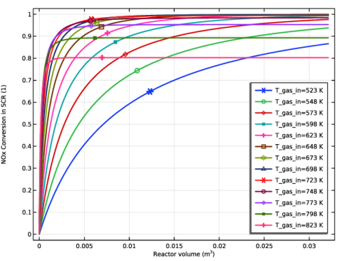
In the Settings window for 1D Plot Group, type Conversion Along Reactor Axis in the Label text field.
2
Click to expand the Title section. From the Title type list, choose None.
3
Locate the Legend section. From the Position list, choose Lower right.
Global 1
1
In the Model Builder window, expand the Conversion Along Reactor Axis node, then click Global 1.
2
In the Settings window for Global, locate the y-Axis Data section.
3
Click  Clear Table.
4
5
Click to expand the Coloring and Style section. From the Color cycle list, choose Long.
6
From the Width list, choose 2.
7
Find the Line markers subsection. From the Marker list, choose Cycle.
8
In the Number text field, type 1.
9
Click to expand the Legends section. Find the Include subsection. Clear the Expression checkbox.
10
Click the  Zoom Extents button in the Graphics toolbar.
11
In the Conversion Along Reactor Axis toolbar, click  Plot.
Temperature (re)
In the Model Builder window, under Results right-click Temperature (re) and choose Delete.
Temperature Increase Along Reactor Axis
1
In the Model Builder window, right-click Conversion Along Reactor Axis and choose Duplicate.
2
In the Model Builder window, click Conversion Along Reactor Axis 1.
3
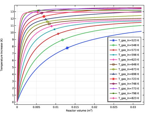
In the Settings window for 1D Plot Group, type Temperature Increase Along Reactor Axis in the Label text field.
Global 1
1
In the Model Builder window, click Global 1.
2
In the Settings window for Global, locate the y-Axis Data section.
3
4
Click the  Zoom Extents button in the Graphics toolbar.
5
In the Temperature Increase Along Reactor Axis toolbar, click  Plot.
Temperature Operating Window
1
In the Results toolbar, click  Evaluation Group.
2
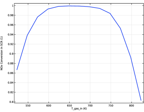
In the Settings window for Evaluation Group, type Temperature Operating Window in the Label text field.
3
Locate the Data section. From the Volume selection list, choose Last.
Global Evaluation 1
1
Right-click Temperature Operating Window and choose Global Evaluation.
2
In the Settings window for Global Evaluation, locate the Expressions section.
3
Click  Clear Table.
4
5
In the Temperature Operating Window toolbar, click  Evaluate.
Temperature Operating Window
1
Go to the Temperature Operating Window window.
2
Click the Table Graph button in the window toolbar.
Results
Table Graph 1
1
In the Settings window for Table Graph, locate the Data section.
2
From the Plot columns list, choose Manual.
3
In the Columns list box, select NOx Conversion in SCR (1).
4
Locate the Coloring and Style section. From the Width list, choose 2.
Temperature Operating Window
1
In the Model Builder window, under Results click 1D Plot Group 3.
2
In the Settings window for 1D Plot Group, type Temperature Operating Window in the Label text field.
3
Click the  Zoom Extents button in the Graphics toolbar.
4
In the Temperature Operating Window toolbar, click  Plot.
For convenience, add the plot groups to a Group with a descriptive name.
Conversion Along Reactor Axis, Temperature Increase Along Reactor Axis, Temperature Operating Window
1
In the Model Builder window, under Results, Ctrl-click to select Conversion Along Reactor Axis, Temperature Increase Along Reactor Axis, and Temperature Operating Window.
2
SCR Temperature Operating Window, ANR = 1.3, Case 2
In the Settings window for Group, type SCR Temperature Operating Window, ANR = 1.3, Case 2 in the Label text field.
Figure 1, Figure 2, and Figure 3 are now done. Continue by investigating the SCR operation as a function of both inlet temperature and ammonia to NOx ratio (ANR). Such a study will generate a lot of data due to the many parameter combinations. Therefore, turn off generate default plots, choose Only plot when requested, and limit the data stored.
Add Study
1
In the Study toolbar, click  Add Study to open the Add Study window.
2
Go to the Add Study window.
3
Find the Studies subsection. In the Select Study tree, select Preset Studies for Selected Physics Interfaces > Stationary Plug Flow.
4
Click the Add Study button in the window toolbar.
5
In the Study toolbar, click  Add Study to close the Add Study window.
Study 2
Step 1: Stationary Plug Flow
In the Model Builder window, under Study 2 right-click Step 1: Stationary Plug Flow and choose Delete.
Study 1: SCR Temperature Operating Window, ANR = 1.3, Case 2
In the Model Builder window, under Study 1: SCR Temperature Operating Window, ANR = 1.3, Case 2 right-click Step 1: Stationary Plug Flow and choose Copy.
Study 2: SCR Temperature Operating Window, ANR Effect, Case 2
In the Model Builder window, right-click Study 2 and choose Paste Stationary Plug Flow.
1
In the Settings window for Stationary Plug Flow, locate the Study Extensions section.
2
3
4
From the Sweep type list, choose All combinations.
5
Locate the Study Settings section. In the Output volumes text field, type range(0, V_SCR/10, V_SCR).
6
In the Model Builder window, click Study 2.
7
In the Settings window for Study, locate the Study Settings section.
8
Clear the Generate default plots checkbox.
9
In the Label text field, type Study 2: SCR Temperature Operating Window, ANR Effect, Case 2.
Solution 2 (sol2)
1
In the Study toolbar, click  Show Default Solver.
2
In the Model Builder window, expand the Solution 2 (sol2) node, then click Dependent Variables 1.
3
In the Settings window for Dependent Variables, locate the Scaling section.
4
From the Method list, choose Initial-value based.
5
In the Model Builder window, under Study 2: SCR Temperature Operating Window, ANR Effect, Case 2 > Solver Configurations > Solution 2 (sol2) click Plug Flow Solver 1.
6
In the Settings window for Plug Flow Solver, locate the General section.
7
From the Volumes to store list, choose Output volumes by interpolation.
Results
1
In the Model Builder window, click Results.
2
In the Settings window for Results, locate the Update of Results section.
3
Select the Only plot when requested checkbox.
Study 2: SCR Temperature Operating Window, ANR Effect, Case 2
In the Study toolbar, click  Compute.
The following steps generate Figure 4.
Results
Temperature Operating Window and ANR Effect, NOx Conversion
1
In the Model Builder window, right-click Temperature Operating Window and choose Duplicate.
2
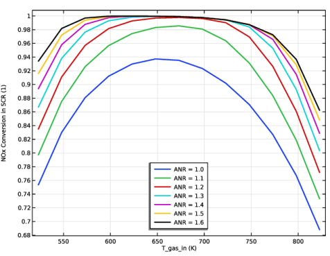
In the Settings window for Evaluation Group, type Temperature Operating Window and ANR Effect, NOx Conversion in the Label text field.
3
Locate the Data section. From the Dataset list, choose None.
Global Evaluation 1
1
In the Model Builder window, expand the Temperature Operating Window and ANR Effect, NOx Conversion node, then click Global Evaluation 1.
2
In the Settings window for Global Evaluation, locate the Data section.
3
From the Dataset list, choose Study 2: SCR Temperature Operating Window, ANR Effect, Case 2/Solution 2 (sol2).
4
From the Parameter selection (ANR) list, choose From list.
5
In the Parameter values (ANR) list box, select 1.
6
From the Volume selection list, choose Last.
7
From the Table columns list, choose ANR.
Global Evaluation 2
1
Right-click Results > Temperature Operating Window and ANR Effect, NOx Conversion > Global Evaluation 1 and choose Duplicate.
2
In the Settings window for Global Evaluation, locate the Data section.
3
In the Parameter values (ANR) list box, select 1.1.
Global Evaluation 3
1
Right-click Global Evaluation 2 and choose Duplicate.
2
In the Settings window for Global Evaluation, locate the Data section.
3
In the Parameter values (ANR) list box, select 1.2.
Global Evaluation 4
1
Right-click Global Evaluation 3 and choose Duplicate.
2
In the Settings window for Global Evaluation, locate the Data section.
3
In the Parameter values (ANR) list box, select 1.3.
Global Evaluation 5
1
Right-click Global Evaluation 4 and choose Duplicate.
2
In the Settings window for Global Evaluation, locate the Data section.
3
In the Parameter values (ANR) list box, select 1.4.
Global Evaluation 6
1
Right-click Global Evaluation 5 and choose Duplicate.
2
In the Settings window for Global Evaluation, locate the Data section.
3
In the Parameter values (ANR) list box, select 1.5.
Global Evaluation 7
1
Right-click Global Evaluation 6 and choose Duplicate.
2
In the Settings window for Global Evaluation, locate the Data section.
3
In the Parameter values (ANR) list box, select 1.6.
Temperature Operating Window and ANR Effect, NOx Conversion
1
In the Model Builder window, click Temperature Operating Window and ANR Effect, NOx Conversion.
2
In the Temperature Operating Window and ANR Effect, NOx Conversion toolbar, click  Evaluate.
Temperature Operating Window and ANR Effect, NOx Conversion
1
Go to the Temperature Operating Window and ANR Effect, NOx Conversion window.
2
Click the Table Graph button in the window toolbar.
Results
ANR = 1.0
1
In the Settings window for Table Graph, type ANR = 1.0 in the Label text field.
2
Locate the Data section. From the Plot columns list, choose Manual.
3
In the Columns list box, select ANR=1, NOx Conversion in SCR (1).
4
Locate the Coloring and Style section. From the Width list, choose 2.
5
Click to expand the Legends section. Select the Show legends checkbox.
6
Find the Include subsection. Select the Label checkbox.
7
Clear the Headers checkbox.
ANR = 1.1
1
Right-click ANR = 1.0 and choose Duplicate.
2
In the Settings window for Table Graph, type ANR = 1.1 in the Label text field.
3
Locate the Data section. In the Columns list box, select ANR=1.1, NOx Conversion in SCR (1).
ANR = 1.2
1
Right-click ANR = 1.1 and choose Duplicate.
2
In the Settings window for Table Graph, type ANR = 1.2 in the Label text field.
3
Locate the Data section. In the Columns list box, select ANR=1.2, NOx Conversion in SCR (1).
ANR = 1.3
1
Right-click ANR = 1.2 and choose Duplicate.
2
In the Settings window for Table Graph, type ANR = 1.3 in the Label text field.
3
Locate the Data section. In the Columns list box, select ANR=1.3, NOx Conversion in SCR (1).
ANR = 1.4
1
Right-click ANR = 1.3 and choose Duplicate.
2
In the Settings window for Table Graph, type ANR = 1.4 in the Label text field.
3
Locate the Data section. In the Columns list box, select ANR=1.4, NOx Conversion in SCR (1).
ANR = 1.5
1
Right-click ANR = 1.4 and choose Duplicate.
2
In the Settings window for Table Graph, type ANR = 1.5 in the Label text field.
3
Locate the Data section. In the Columns list box, select ANR=1.5, NOx Conversion in SCR (1).
ANR = 1.6
1
Right-click ANR = 1.5 and choose Duplicate.
2
In the Settings window for Table Graph, type ANR = 1.6 in the Label text field.
3
Locate the Data section. In the Columns list box, select ANR=1.6, NOx Conversion in SCR (1).
NOx Conversion in SCR
1
In the Model Builder window, under Results click 1D Plot Group 4.
2
In the Settings window for 1D Plot Group, type NOx Conversion in SCR in the Label text field.
3
Locate the Plot Settings section.
4
Select the y-axis label checkbox. In the associated text field, type NOx Conversion in SCR (1).
5
Locate the Legend section. From the Position list, choose Lower middle.
6
Click the  Zoom Extents button in the Graphics toolbar.
7
In the NOx Conversion in SCR toolbar, click  Plot.
The following steps generate Figure 5.
Temperature Operating Window and ANR Effect, NH3 Conversion
1
In the Model Builder window, right-click Temperature Operating Window and ANR Effect, NOx Conversion and choose Duplicate.
2
In the Model Builder window, click Temperature Operating Window and ANR Effect, NOx Conversion 1.
3
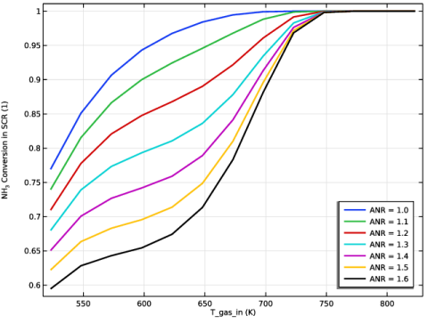
In the Settings window for Evaluation Group, type Temperature Operating Window and ANR Effect, NH3 Conversion in the Label text field.
Global Evaluation 1
1
In the Model Builder window, click Global Evaluation 1.
2
In the Settings window for Global Evaluation, locate the Expressions section.
3
Global Evaluation 2
1
In the Model Builder window, click Global Evaluation 2.
2
In the Settings window for Global Evaluation, locate the Expressions section.
3
Global Evaluation 3
1
In the Model Builder window, click Global Evaluation 3.
2
In the Settings window for Global Evaluation, locate the Expressions section.
3
Global Evaluation 4
1
In the Model Builder window, click Global Evaluation 4.
2
In the Settings window for Global Evaluation, locate the Expressions section.
3
Global Evaluation 5
1
In the Model Builder window, click Global Evaluation 5.
2
In the Settings window for Global Evaluation, locate the Expressions section.
3
Global Evaluation 6
1
In the Model Builder window, click Global Evaluation 6.
2
In the Settings window for Global Evaluation, locate the Expressions section.
3
Global Evaluation 7
1
In the Model Builder window, click Global Evaluation 7.
2
In the Settings window for Global Evaluation, locate the Expressions section.
3
Temperature Operating Window and ANR Effect, NH3 Conversion
1
In the Model Builder window, click Temperature Operating Window and ANR Effect, NH3 Conversion.
2
In the Temperature Operating Window and ANR Effect, NH3 Conversion toolbar, click  Evaluate.
NH3 Conversion in SCR
1
In the Model Builder window, right-click NOx Conversion in SCR and choose Duplicate.
2
In the Model Builder window, click NOx Conversion in SCR 1.
3
In the Settings window for 1D Plot Group, type NH3 Conversion in SCR in the Label text field.
4
Locate the Plot Settings section.
5
Select the y-axis label checkbox. In the associated text field, type NH<sub>3</sub> Conversion in SCR (1).
6
Locate the Legend section. From the Position list, choose Lower right.
ANR = 1.0
1
In the Model Builder window, click ANR = 1.0.
2
In the Settings window for Table Graph, locate the Data section.
3
From the Evaluation group list, choose Temperature Operating Window and ANR Effect, NH3 Conversion.
ANR = 1.1
1
In the Model Builder window, click ANR = 1.1.
2
In the Settings window for Table Graph, locate the Data section.
3
From the Evaluation group list, choose Temperature Operating Window and ANR Effect, NH3 Conversion.
ANR = 1.2
1
In the Model Builder window, click ANR = 1.2.
2
In the Settings window for Table Graph, locate the Data section.
3
From the Evaluation group list, choose Temperature Operating Window and ANR Effect, NH3 Conversion.
ANR = 1.3
1
In the Model Builder window, click ANR = 1.3.
2
In the Settings window for Table Graph, locate the Data section.
3
From the Evaluation group list, choose Temperature Operating Window and ANR Effect, NH3 Conversion.
ANR = 1.4
1
In the Model Builder window, click ANR = 1.4.
2
In the Settings window for Table Graph, locate the Data section.
3
From the Evaluation group list, choose Temperature Operating Window and ANR Effect, NH3 Conversion.
ANR = 1.5
1
In the Model Builder window, click ANR = 1.5.
2
In the Settings window for Table Graph, locate the Data section.
3
From the Evaluation group list, choose Temperature Operating Window and ANR Effect, NH3 Conversion.
ANR = 1.6
1
In the Model Builder window, click ANR = 1.6.
2
In the Settings window for Table Graph, locate the Data section.
3
From the Evaluation group list, choose Temperature Operating Window and ANR Effect, NH3 Conversion.
4
Click the  Zoom Extents button in the Graphics toolbar.
5
In the NH3 Conversion in SCR toolbar, click  Plot.
NH3 Conversion in SCR, NOx Conversion in SCR
1
In the Model Builder window, under Results, Ctrl-click to select NOx Conversion in SCR and NH3 Conversion in SCR.
2
SCR Temperature Operating Window and ANR Effect, Case 2
1
In the Settings window for Group, type SCR Temperature Operating Window and ANR Effect, Case 2 in the Label text field.
We have now investigated the influence of both inlet temperature and ammonia to NOx ratio on the SCR monolith system. Now solve for both of the catalysts in series. Begin by turning off the functionality to only plot when requested.
2
In the Model Builder window, click Results.
3
In the Settings window for Results, locate the Update of Results section.
4
Clear the Only plot when requested checkbox.
Add Study
1
In the Home toolbar, click  Add Study to open the Add Study window.
2
Go to the Add Study window.
3
Find the Studies subsection. In the Select Study tree, select Preset Studies for Selected Physics Interfaces > Stationary Plug Flow.
4
Click the Add Study button in the window toolbar.
5
In the Home toolbar, click  Add Study to close the Add Study window.
Study 3
Stationary Plug Flow, SCR
1
In the Settings window for Stationary Plug Flow, type Stationary Plug Flow, SCR in the Label text field.
2
Locate the Study Settings section. In the Output volumes text field, type 0 V_SCR.
3
Locate the Physics and Variables Selection section. In the Solve for column of the table, under Component 1 (comp1), clear the checkbox for Ammonia Slip Catalyst (ASC) (re2).
Stationary Plug Flow, ASC
1
Right-click Study 3 > Step 1: Stationary Plug Flow, SCR and choose Duplicate.
2
In the Settings window for Stationary Plug Flow, type Stationary Plug Flow, ASC in the Label text field.
3
Locate the Study Settings section. In the Output volumes text field, type V_SCR V_SCR+V_ASC.
4
Locate the Physics and Variables Selection section. In the Solve for column of the table, under Component 1 (comp1), select the checkbox for Ammonia Slip Catalyst (ASC) (re2).
5
In the Solve for column of the table, under Component 1 (comp1), clear the checkbox for Selective Catalytic Reduction Catalyst (SCR) (re).
To connect the two beds we need to create the dataset for the study.
6
In the Model Builder window, click Study 3.
7
In the Settings window for Study, type Study 3: Single Channel Model, Influence of ANR, Case 2 in the Label text field.
8
Locate the Study Settings section. Select the Store solution for all intermediate study steps checkbox.
9
Clear the Generate default plots checkbox.
10
In the Study toolbar, click  Get Initial Value.
We can now connect the two Reaction Engineering interfaces with each other, so that the second catalyst uses the output from the first catalyst as input.
11
In the Model Builder window, click Step 2: Stationary Plug Flow, ASC.
12
In the Settings window for Stationary Plug Flow, click to expand the Values of Dependent Variables section.
13
Find the Initial values of variables solved for subsection. From the Settings list, choose User controlled.
14
From the Method list, choose Initial expression.
15
From the Selection list, choose Last.
16
Find the Values of variables not solved for subsection. From the Settings list, choose User controlled.
17
From the Selection list, choose Last.
Use initial value based scales for the dependent variables.
Solver Configurations
In the Model Builder window, expand the Study 3: Single Channel Model, Influence of ANR, Case 2 > Solver Configurations node.
Solution 3 (sol3)
1
In the Model Builder window, expand the Study 3: Single Channel Model, Influence of ANR, Case 2 > Solver Configurations > Solution 3 (sol3) node, then click Dependent Variables 1.
2
In the Settings window for Dependent Variables, locate the Scaling section.
3
From the Method list, choose Initial-value based.
4
In the Model Builder window, click Dependent Variables 2.
5
In the Settings window for Dependent Variables, locate the Scaling section.
6
From the Method list, choose Initial-value based.
Add a Parametric Sweep feature to solve for three different ammonia to NOx ratios.
Parametric Sweep
1
In the Study toolbar, click  Parametric Sweep.
2
In the Settings window for Parametric Sweep, locate the Study Settings section.
3
4
5
In the Study toolbar, click  Compute.
The following steps generate Figure 6.
Results
Molar Fraction of NH3 and NOx
1
In the Results toolbar, click  1D Plot Group.
2
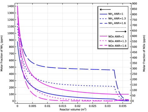
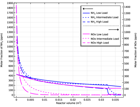
In the Settings window for 1D Plot Group, type Molar Fraction of NH3 and NOx in the Label text field.
3
Locate the Data section. From the Dataset list, choose Study 3: Single Channel Model, Influence of ANR, Case 2/Parametric Solutions 2 (sol6).
NH3 SCR
1
Right-click Molar Fraction of NH3 and NOx and choose Global.
2
In the Settings window for Global, type NH3 SCR in the Label text field.
3
Locate the y-Axis Data section. Click  Clear Table.
4
Click Replace Expression in the upper-right corner of the y-Axis Data section. From the menu, choose Component 1 (comp1) > Definitions > Variables > yNH3_SCR - Molar fraction of NH3 in SCR catalytic bed - 1.
5
Locate the y-Axis Data section. In the table, enter the following settings:
6
Locate the Coloring and Style section. Find the Line style subsection. From the Line list, choose Cycle.
7
From the Color list, choose Blue.
8
From the Width list, choose 2.
9
Locate the Legends section. Clear the Show legends checkbox.
NH3
1
Right-click NH3 SCR and choose Duplicate.
2
In the Settings window for Global, type NH3 in the Label text field.
3
Locate the Data section. From the Dataset list, choose Study 3: Single Channel Model, Influence of ANR, Case 2/Parametric Solutions 1 (sol5).
4
Locate the y-Axis Data section. In the table, enter the following settings:
5
Locate the Coloring and Style section. Find the Line style subsection. From the Line list, choose Cycle (reset).
6
Locate the Legends section. Select the Show legends checkbox.
7
Find the Include subsection. Clear the Expression checkbox.
8
Find the Prefix and suffix subsection. In the Prefix text field, type NH<sub>3</sub> .
NOx SCR
1
In the Model Builder window, right-click NH3 SCR and choose Duplicate.
2
In the Settings window for Global, type NOx SCR in the Label text field.
3
Locate the y-Axis Data section. In the table, enter the following settings:
4
Locate the Coloring and Style section. Find the Line style subsection. From the Line list, choose Cycle (reset).
5
From the Color list, choose Magenta.
NOx
1
Right-click NOx SCR and choose Duplicate.
2
In the Settings window for Global, type NOx in the Label text field.
3
Locate the Data section. From the Dataset list, choose Study 3: Single Channel Model, Influence of ANR, Case 2/Parametric Solutions 1 (sol5).
4
Locate the y-Axis Data section. In the table, enter the following settings:
5
Locate the Legends section. Select the Show legends checkbox.
6
Find the Include subsection. Select the Label checkbox.
7
Clear the Expression checkbox.
Molar Fraction of NH3 and NOx
1
In the Model Builder window, click Molar Fraction of NH3 and NOx.
2
In the Settings window for 1D Plot Group, locate the Title section.
3
From the Title type list, choose None.
4
Locate the Plot Settings section.
5
Select the x-axis label checkbox. In the associated text field, type Reactor volume (m<sup>3</sup>).
6
Select the y-axis label checkbox. In the associated text field, type Molar Fraction of NH<sub>3</sub> (ppm).
7
Select the Two y-axes checkbox.
8
9
Select the Secondary y-axis label checkbox. In the associated text field, type Molar Fraction of NOx (ppm).
10
Click the  Zoom Extents button in the Graphics toolbar.
11
In the Molar Fraction of NH3 and NOx toolbar, click  Plot.
The following steps generate Figure 7.
Conversion of NH3 and NOx
1
Right-click Molar Fraction of NH3 and NOx and choose Duplicate.
2
In the Model Builder window, click Molar Fraction of NH3 and NOx 1.
3
In the Settings window for 1D Plot Group, type Conversion of NH3 and NOx in the Label text field.
4
Locate the Plot Settings section. In the y-axis label text field, type Conversion (1).
5
Clear the Two y-axes checkbox.
6
Locate the Legend section. From the Position list, choose Lower right.
NH3 SCR
1
In the Model Builder window, click NH3 SCR.
2
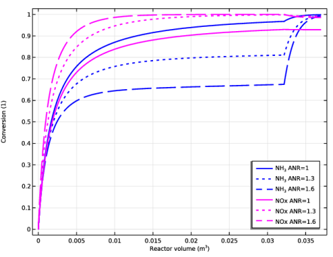
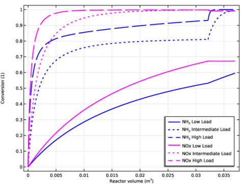
In the Settings window for Global, click Replace Expression in the upper-right corner of the y-Axis Data section. From the menu, choose Component 1 (comp1) > Definitions > Variables > X_NH3_SCR - NH3 Conversion in SCR - 1.
3
Locate the y-Axis Data section. In the table, enter the following settings:
NH3
1
In the Model Builder window, click NH3.
2
In the Settings window for Global, locate the y-Axis Data section.
3
NOx SCR
1
In the Model Builder window, click NOx SCR.
2
In the Settings window for Global, locate the y-Axis Data section.
3
NOx
1
In the Model Builder window, click NOx.
2
In the Settings window for Global, locate the y-Axis Data section.
3
4
Click the  Zoom Extents button in the Graphics toolbar.
5
In the Conversion of NH3 and NOx toolbar, click  Plot.
The intermediate engine load case, referred to as case 2, has now been investigated, both in terms of temperature and ANR. How well does the system perform for other engine loads? Add a final study to investigate three different load cases for an ANR = 1.3.
Conversion of NH3 and NOx, Molar Fraction of NH3 and NOx
1
In the Model Builder window, under Results, Ctrl-click to select Molar Fraction of NH3 and NOx and Conversion of NH3 and NOx.
2
Single Channel Model, Influence of ANR, Case 2
In the Settings window for Group, type Single Channel Model, Influence of ANR, Case 2 in the Label text field.
Add Study
1
In the Home toolbar, click  Add Study to open the Add Study window.
2
Go to the Add Study window.
3
Find the Studies subsection. In the Select Study tree, select Preset Studies for Selected Physics Interfaces > Stationary Plug Flow.
4
Click the Add Study button in the window toolbar.
5
In the Home toolbar, click  Add Study to close the Add Study window.
Study 4
Step 1: Stationary Plug Flow
In the Model Builder window, under Study 4 right-click Step 1: Stationary Plug Flow and choose Delete.
Study 3: Single Channel Model, Influence of ANR, Case 2
Parametric Sweep, Step 1: Stationary Plug Flow, SCR, Step 2: Stationary Plug Flow, ASC
1
In the Model Builder window, under Study 3: Single Channel Model, Influence of ANR, Case 2, Ctrl-click to select Parametric Sweep, Step 1: Stationary Plug Flow, SCR, and Step 2: Stationary Plug Flow, ASC.
2
Study 4: Single Channel Model, ANR = 1.3, All Cases
1
In the Model Builder window, right-click Study 4 and choose Paste Multiple Items.
2
In the Settings window for Study, type Study 4: Single Channel Model, ANR = 1.3, All Cases in the Label text field.
3
Locate the Study Settings section. Select the Store solution for all intermediate study steps checkbox.
4
Clear the Generate default plots checkbox.
Parametric Sweep
1
In the Model Builder window, under Study 4: Single Channel Model, ANR = 1.3, All Cases click Parametric Sweep.
2
In the Settings window for Parametric Sweep, locate the Study Settings section.
3
From the Sweep type list, choose Parameter switch.
4
5
Use initial value based scales for the dependent variables.
Solution 13 (sol13)
1
In the Study toolbar, click  Show Default Solver.
2
In the Model Builder window, expand the Solution 13 (sol13) node, then click Dependent Variables 1.
3
In the Settings window for Dependent Variables, locate the Scaling section.
4
From the Method list, choose Initial-value based.
5
In the Model Builder window, under Study 4: Single Channel Model, ANR = 1.3, All Cases > Solver Configurations > Solution 13 (sol13) click Dependent Variables 2.
6
In the Settings window for Dependent Variables, locate the Scaling section.
7
From the Method list, choose Initial-value based.
Step 2: Stationary Plug Flow, ASC
1
In the Model Builder window, under Study 4: Single Channel Model, ANR = 1.3, All Cases click Step 2: Stationary Plug Flow, ASC.
2
In the Settings window for Stationary Plug Flow, locate the Values of Dependent Variables section.
3
Find the Initial values of variables solved for subsection. From the Study list, choose Study 4: Single Channel Model, ANR = 1.3, All Cases, Stationary Plug Flow, SCR.
4
From the Use list, choose Solution Store 2 (sol14).
5
Find the Values of variables not solved for subsection. From the Study list, choose Study 4: Single Channel Model, ANR = 1.3, All Cases, Stationary Plug Flow, SCR.
6
From the Use list, choose Solution Store 2 (sol14).
7
In the Study toolbar, click  Compute.
The following steps generate Figure 8 and Figure 9.
Results
Single Channel Model, ANR = 1.3, All Cases
1
In the Model Builder window, right-click Single Channel Model, Influence of ANR, Case 2 and choose Duplicate.
2
In the Settings window for Group, type Single Channel Model, ANR = 1.3, All Cases in the Label text field.
Molar Fraction of NH3 and NOx, All Cases
1
In the Model Builder window, expand the Single Channel Model, ANR = 1.3, All Cases node, then click Molar Fraction of NH3 and NOx 1.
2
In the Settings window for 1D Plot Group, type Molar Fraction of NH3 and NOx, All Cases in the Label text field.
3
Locate the Data section. From the Dataset list, choose Study 4: Single Channel Model, ANR = 1.3, All Cases/Parametric Solutions 4 (sol16).
NH3
1
In the Model Builder window, expand the Molar Fraction of NH3 and NOx, All Cases node, then click NH3.
2
In the Settings window for Global, locate the Data section.
3
From the Dataset list, choose Study 4: Single Channel Model, ANR = 1.3, All Cases/Parametric Solutions 3 (sol15).
NOx
1
In the Model Builder window, click NOx.
2
In the Settings window for Global, locate the Data section.
3
From the Dataset list, choose Study 4: Single Channel Model, ANR = 1.3, All Cases/Parametric Solutions 3 (sol15).
4
Click the  Zoom Extents button in the Graphics toolbar.
5
In the Molar Fraction of NH3 and NOx, All Cases toolbar, click  Plot.
Conversion of NH3 and NOx, All Cases
1
In the Model Builder window, under Results > Single Channel Model, ANR = 1.3, All Cases click Conversion of NH3 and NOx 1.
2
In the Settings window for 1D Plot Group, type Conversion of NH3 and NOx, All Cases in the Label text field.
3
Locate the Data section. From the Dataset list, choose Study 4: Single Channel Model, ANR = 1.3, All Cases/Parametric Solutions 4 (sol16).
NH3
1
In the Model Builder window, expand the Conversion of NH3 and NOx, All Cases node, then click NH3.
2
In the Settings window for Global, locate the Data section.
3
From the Dataset list, choose Study 4: Single Channel Model, ANR = 1.3, All Cases/Parametric Solutions 3 (sol15).
NOx
1
In the Model Builder window, click NOx.
2
In the Settings window for Global, locate the Data section.
3
From the Dataset list, choose Study 4: Single Channel Model, ANR = 1.3, All Cases/Parametric Solutions 3 (sol15).
4
Click the  Zoom Extents button in the Graphics toolbar.
5
In the Conversion of NH3 and NOx, All Cases toolbar, click  Plot.
The following steps generate Figure 10.
Temperature Increase Along Reactor Axis, All Cases
1
In the Model Builder window, right-click Conversion of NH3 and NOx, All Cases and choose Duplicate.
2
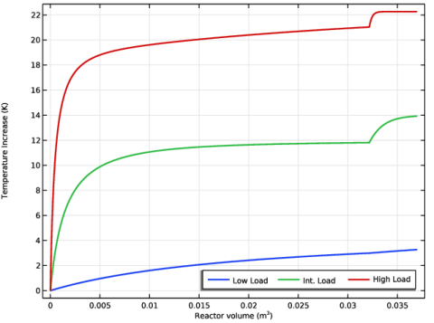
In the Settings window for 1D Plot Group, type Temperature Increase Along Reactor Axis, All Cases in the Label text field.
3
Locate the Plot Settings section. In the y-axis label text field, type Temperature Increase (K).
4
In the Model Builder window, expand the Temperature Increase Along Reactor Axis, All Cases node.
NOx, NOx SCR
1
In the Model Builder window, under Results > Single Channel Model, ANR = 1.3, All Cases > Temperature Increase Along Reactor Axis, All Cases, Ctrl-click to select NOx SCR and NOx.
2
Temperature Increase SCR
1
In the Model Builder window, under Results > Single Channel Model, ANR = 1.3, All Cases > Temperature Increase Along Reactor Axis, All Cases click NH3 SCR.
2
In the Settings window for Global, type Temperature Increase SCR in the Label text field.
3
Locate the y-Axis Data section. In the table, enter the following settings:
4
Locate the Coloring and Style section. Find the Line style subsection. From the Line list, choose Solid.
5
From the Color list, choose Cycle.
Temperature Increase ASC
1
In the Model Builder window, under Results > Single Channel Model, ANR = 1.3, All Cases > Temperature Increase Along Reactor Axis, All Cases click NH3.
2
In the Settings window for Global, type Temperature Increase ASC in the Label text field.
3
Locate the y-Axis Data section. In the table, enter the following settings:
4
Locate the Coloring and Style section. Find the Line style subsection. From the Line list, choose Solid.
5
From the Color list, choose Cycle (reset).
6
Click to expand the Legends section. From the Legends list, choose Manual.
7
Temperature Increase Along Reactor Axis, All Cases
1
In the Model Builder window, click Temperature Increase Along Reactor Axis, All Cases.
2
In the Settings window for 1D Plot Group, locate the Legend section.
3
In the Number of columns text field, type 3.
4
In the Maximum relative width text field, type 1.
5
Click the  Zoom Extents button in the Graphics toolbar.
6
In the Temperature Increase Along Reactor Axis, All Cases toolbar, click  Plot.