
|
|
|
 ,
,
|
1
|
|
2
|
|
3
|
Click Add.
|
|
4
|
|
5
|
In the Velocity field components table, enter the following settings:
|
|
6
|
|
7
|
In the Select Physics tree, select Mathematics > ODE and DAE Interfaces > Domain ODEs and DAEs (dode).
|
|
8
|
Click Add.
|
|
9
|
|
10
|
In the Dependent variables (1) table, enter the following settings:
|
|
11
|
Click
|
|
12
|
In the Source term quantity table, enter the following settings:
|
|
13
|
In the Select Physics tree, select Chemical Species Transport > Nonisothermal Reacting Flow > Porous Media Flow > Brinkman Equations.
|
|
14
|
Click Add.
|
|
15
|
In the Added physics interfaces tree, select Transport of Concentrated Species in Porous Media (tcs).
|
|
16
|
In the Mass fractions (1) table, enter the following settings:
|
|
17
|
Click
|
|
18
|
|
19
|
Click
|
|
1
|
|
2
|
|
3
|
|
4
|
Browse to the model’s Application Libraries folder and double-click the file metal_hydride_tank_parameters.txt.
|
|
1
|
|
2
|
|
3
|
|
4
|
Browse to the model’s Application Libraries folder and double-click the file metal_hydride_tank_kinetic_parameters.txt.
|
|
1
|
|
2
|
In the Settings window for Interpolation, type p_iso(Tiso,XH) (Experimental pressure-composition-isotherm curve at 20 degC) in the Label text field.
|
|
3
|
|
4
|
Click
|
|
5
|
Browse to the model’s Application Libraries folder and double-click the file metal_hydride_tank_PCI_curve.txt.
|
|
6
|
|
7
|
|
8
|
In the Argument table, enter the following settings:
|
|
1
|
|
2
|
In the Settings window for Analytic, type p_eq(T,XH) (Equilibrium Hydrogen Pressure) in the Label text field.
|
|
3
|
|
4
|
Locate the Definition section. In the Expression text field, type p_iso(XH)*exp(deltaH/R_const*(1/T-1/293.15[K])).
|
|
5
|
|
6
|
|
1
|
|
2
|
Browse to the model’s Application Libraries folder and double-click the file metal_hydride_tank_geom_sequence.mph.
|
|
3
|
|
1
|
|
2
|
Go to the Add Material window.
|
|
3
|
|
4
|
Click Search.
|
|
5
|
|
6
|
Click the Add to Component button in the window toolbar.
|
|
7
|
|
1
|
|
2
|
|
1
|
|
2
|
|
3
|
|
4
|
In the Model Builder window, expand the Component 1 (comp1) > Materials > Gas Mixture (mat2) node, then click Basic (def).
|
|
5
|
|
6
|
Click
|
|
7
|
|
8
|
|
9
|
Click OK.
|
|
10
|
|
12
|
Click
|
|
13
|
|
14
|
|
15
|
Click OK.
|
|
16
|
|
18
|
Click
|
|
19
|
|
20
|
|
21
|
Click OK.
|
|
22
|
|
1
|
|
2
|
|
3
|
|
1
|
|
2
|
|
3
|
|
1
|
|
2
|
|
3
|
|
4
|
|
5
|
|
6
|
Click
|
|
7
|
|
8
|
|
9
|
Click OK.
|
|
10
|
|
12
|
Click
|
|
13
|
|
14
|
|
15
|
Click OK.
|
|
16
|
|
18
|
Click
|
|
19
|
|
20
|
|
21
|
Click OK.
|
|
22
|
|
24
|
|
1
|
|
2
|
|
3
|
Click
|
|
4
|
|
5
|
|
6
|
Click OK.
|
|
7
|
|
1
|
|
2
|
Go to the Add Material window.
|
|
3
|
|
4
|
Click Search.
|
|
5
|
|
6
|
Click the Add to Component button in the window toolbar.
|
|
7
|
|
1
|
|
2
|
|
1
|
|
2
|
|
3
|
|
4
|
|
5
|
Browse to the model’s Application Libraries folder and double-click the file metal_hydride_tank_variables.txt.
|
|
1
|
|
2
|
|
3
|
|
4
|
|
1
|
|
2
|
|
3
|
|
4
|
|
1
|
|
2
|
|
3
|
|
4
|
Click Apply.
|
|
5
|
|
6
|
Locate the Reaction Thermodynamic Properties section. From the Enthalpy of reaction list, choose User defined.
|
|
7
|
|
1
|
|
2
|
|
3
|
|
4
|
|
5
|
|
6
|
|
1
|
|
2
|
|
3
|
|
4
|
|
5
|
|
6
|
|
7
|
|
8
|
|
9
|
|
10
|
Find the Bulk species subsection. From the Species solved for list, choose Transport of Concentrated Species in Porous Media.
|
|
12
|
Click to expand the Calculate Transport Properties section. From the Ratio of specific heats list, choose User defined.
|
|
13
|
|
14
|
|
15
|
|
1
|
|
2
|
In the Settings window for Domain ODEs and DAEs, type Absorbed Hydrogen Atoms Per Metal Atom, XH in the Label text field.
|
|
3
|
|
4
|
|
5
|
|
6
|
|
1
|
In the Model Builder window, under Component 1 (comp1) > Absorbed Hydrogen Atoms Per Metal Atom, XH (dode) click Distributed ODE 1.
|
|
2
|
|
3
|
|
1
|
|
2
|
|
3
|
|
1
|
|
2
|
|
3
|
|
4
|
Locate the Physical Model section. From the Compressibility list, choose Compressible flow (Ma<0.3).
|
|
5
|
Clear the Neglect inertial term (Stokes flow) checkbox.
|
|
6
|
|
7
|
|
1
|
|
2
|
|
3
|
|
1
|
In the Model Builder window, under Component 1 (comp1) > Brinkman Equations (br) > Porous Medium 1 click Porous Matrix 1.
|
|
2
|
|
3
|
|
4
|
|
1
|
|
2
|
|
3
|
From the list, choose Pressure.
|
|
4
|
|
5
|
|
1
|
|
2
|
|
3
|
|
1
|
In the Model Builder window, under Component 1 (comp1) > Heat Transfer in Porous Media (ht) click Porous Medium 1.
|
|
2
|
|
3
|
|
1
|
|
2
|
|
3
|
|
1
|
|
2
|
|
3
|
|
1
|
|
2
|
|
3
|
|
1
|
|
2
|
|
3
|
|
4
|
|
1
|
|
2
|
|
3
|
|
4
|
|
5
|
|
6
|
|
1
|
|
2
|
|
3
|
|
1
|
|
2
|
|
3
|
|
4
|
Locate the Model Input section. Click Make All Model Inputs Editable in the upper-right corner of the section.
|
|
5
|
|
6
|
|
7
|
|
1
|
|
2
|
|
3
|
|
4
|
Locate the Upstream Properties section. In the Tustr text field, type Tcooling*step2(t)+T0*(1-step2(t)).
|
|
1
|
|
2
|
|
3
|
|
1
|
In the Model Builder window, under Component 1 (comp1) click Transport of Concentrated Species in Porous Media (tcs).
|
|
2
|
In the Settings window for Transport of Concentrated Species in Porous Media, locate the Domain Selection section.
|
|
3
|
|
1
|
In the Model Builder window, under Component 1 (comp1) > Transport of Concentrated Species in Porous Media (tcs) > Porous Medium 1 click Fluid 1.
|
|
2
|
|
4
|
|
1
|
In the Model Builder window, under Component 1 (comp1) > Transport of Concentrated Species in Porous Media (tcs) click Initial Values 1.
|
|
2
|
|
3
|
|
4
|
|
1
|
|
2
|
|
4
|
|
1
|
|
2
|
|
3
|
|
4
|
|
5
|
Select the Mass transfer to other phases checkbox.
|
|
1
|
|
2
|
|
3
|
|
4
|
|
5
|
|
1
|
|
2
|
|
3
|
|
1
|
|
2
|
|
3
|
|
1
|
|
2
|
|
3
|
|
4
|
|
5
|
|
1
|
|
2
|
|
3
|
|
1
|
|
2
|
|
3
|
|
4
|
|
5
|
In the Show More Options dialog, in the tree, select the checkbox for the node Physics > Advanced Physics Options.
|
|
6
|
Click OK.
|
|
7
|
|
8
|
|
9
|
Find the Pseudo time stepping subsection. From the Use pseudo time stepping for stationary equation form list, choose On.
|
|
1
|
|
2
|
|
3
|
|
4
|
|
1
|
|
2
|
|
3
|
|
4
|
|
1
|
|
2
|
|
3
|
|
4
|
|
5
|
|
6
|
|
7
|
Click the Custom button.
|
|
8
|
Locate the Element Size Parameters section.
|
|
9
|
|
10
|
|
11
|
Select the Maximum element growth rate checkbox.
|
|
12
|
Select the Curvature factor checkbox.
|
|
13
|
Select the Resolution of narrow regions checkbox.
|
|
14
|
Click
|
|
1
|
|
2
|
|
3
|
|
4
|
|
5
|
|
6
|
|
7
|
|
8
|
Click the Custom button.
|
|
9
|
Locate the Element Size Parameters section.
|
|
10
|
|
11
|
Click
|
|
1
|
|
2
|
|
3
|
|
4
|
|
5
|
Clear the Minimum element size checkbox.
|
|
6
|
|
7
|
Clear the Curvature factor checkbox.
|
|
8
|
Clear the Resolution of narrow regions checkbox.
|
|
9
|
|
10
|
Click
|
|
1
|
|
2
|
|
3
|
|
5
|
|
6
|
|
7
|
Click the Custom button.
|
|
8
|
Locate the Element Size Parameters section.
|
|
9
|
|
10
|
|
11
|
Select the Maximum element growth rate checkbox.
|
|
12
|
Select the Curvature factor checkbox.
|
|
13
|
Select the Resolution of narrow regions checkbox.
|
|
14
|
Click
|
|
1
|
|
1
|
|
3
|
|
4
|
|
1
|
|
3
|
|
4
|
|
5
|
|
6
|
|
7
|
Click
|
|
1
|
|
1
|
|
3
|
|
4
|
|
1
|
|
3
|
|
4
|
|
5
|
|
6
|
|
7
|
Select the Symmetric distribution checkbox.
|
|
8
|
Click
|
|
1
|
|
1
|
|
3
|
|
4
|
|
1
|
|
3
|
|
4
|
|
5
|
|
6
|
|
7
|
Select the Symmetric distribution checkbox.
|
|
8
|
Click
|
|
1
|
|
1
|
|
2
|
|
3
|
|
4
|
Click the Custom button.
|
|
5
|
|
6
|
Click in the Maximum element size text field, then press Ctrl+Space. From the menu, choose Parameters > dCoolingChannel - Thickness, cooling channel - m.
|
|
7
|
|
8
|
|
9
|
Select the Maximum element growth rate checkbox.
|
|
10
|
Select the Curvature factor checkbox.
|
|
11
|
Select the Resolution of narrow regions checkbox.
|
|
12
|
Click
|
|
1
|
|
2
|
|
3
|
|
1
|
|
2
|
|
3
|
|
4
|
Click
|
|
1
|
|
2
|
|
3
|
|
4
|
|
5
|
Click
|
|
1
|
|
2
|
|
3
|
|
4
|
|
1
|
|
2
|
|
3
|
|
4
|
Click
|
|
1
|
|
2
|
|
1
|
|
2
|
|
3
|
|
1
|
In the Model Builder window, expand the Boundary Layers 1 node, then click Boundary Layer Properties 1.
|
|
2
|
|
3
|
|
1
|
|
2
|
|
3
|
|
4
|
Click
|
|
1
|
In the Model Builder window, under Component 1 (comp1) > Mesh 1 right-click Boundary Layers 1 and choose Duplicate.
|
|
2
|
|
3
|
|
1
|
In the Model Builder window, expand the Boundary Layers 2 node, then click Boundary Layer Properties 1.
|
|
2
|
|
3
|
|
4
|
|
5
|
Click
|
|
1
|
|
2
|
|
3
|
|
1
|
In the Model Builder window, expand the Boundary Layers 3 node, then click Boundary Layer Properties 1.
|
|
2
|
|
3
|
|
4
|
|
5
|
|
6
|
Click
|
|
1
|
|
2
|
|
1
|
|
2
|
|
3
|
In the Solve for column of the table, under Component 1 (comp1), clear the checkboxes for Absorbed Hydrogen Atoms Per Metal Atom, XH (dode), Chemistry (chem), Transport of Concentrated Species in Porous Media (tcs), Brinkman Equations (br), and Heat Transfer in Porous Media (ht).
|
|
4
|
In the Solve for column of the table, under Component 1 (comp1) > Multiphysics, clear the checkbox for Reacting Flow 1 (nirf1).
|
|
5
|
|
1
|
|
2
|
|
3
|
|
4
|
|
5
|
Locate the Coloring and Style section. Find the Line style subsection. From the Type list, choose Tube.
|
|
6
|
|
7
|
Select the Radius scale factor checkbox.
|
|
8
|
|
1
|
|
2
|
|
3
|
|
1
|
|
1
|
|
2
|
Clear the Plot dataset edges checkbox.
|
|
3
|
|
1
|
|
2
|
Right-click and choose Group.
|
|
1
|
|
2
|
Drag and drop below Tables.
|
|
1
|
|
2
|
Go to the Add Study window.
|
|
3
|
|
4
|
Click the Add Study button in the window toolbar.
|
|
5
|
|
1
|
|
2
|
|
3
|
|
4
|
Locate the Physics and Variables Selection section. In the Solve for column of the table, under Component 1 (comp1), clear the checkbox for Laminar Flow - Cooling (spf).
|
|
5
|
Click to expand the Values of Dependent Variables section. Find the Values of variables not solved for subsection. From the Settings list, choose User controlled.
|
|
6
|
|
7
|
|
8
|
|
9
|
|
10
|
Clear the Generate default plots checkbox.
|
|
11
|
|
1
|
|
2
|
|
3
|
In the Model Builder window, expand the Study 2: Absorption > Solver Configurations > Solution 2 (sol2) > Dependent Variables 1 node, then click Pressure (comp1.p).
|
|
4
|
|
5
|
|
6
|
|
7
|
|
8
|
|
9
|
|
10
|
|
11
|
|
12
|
|
13
|
|
14
|
|
15
|
|
16
|
|
17
|
|
18
|
|
19
|
|
20
|
|
21
|
|
22
|
|
23
|
|
24
|
Click to expand the Time Stepping section.
|
|
25
|
|
1
|
|
2
|
|
3
|
Select the Only plot when requested checkbox.
|
|
4
|
|
1
|
|
2
|
|
3
|
|
4
|
|
5
|
|
6
|
|
7
|
|
8
|
|
9
|
|
10
|
|
1
|
|
2
|
|
3
|
|
4
|
|
1
|
|
2
|
In the Settings window for Surface, click Replace Expression in the upper-right corner of the Expression section. From the menu, choose Component 1 (comp1) > Brinkman Equations > Velocity and pressure > br.U - Velocity magnitude - m/s.
|
|
3
|
|
4
|
|
5
|
|
6
|
|
1
|
|
2
|
|
3
|
|
4
|
|
5
|
|
6
|
|
7
|
|
8
|
|
1
|
|
2
|
|
3
|
|
1
|
|
2
|
|
3
|
|
1
|
|
2
|
|
3
|
|
4
|
|
5
|
|
6
|
|
1
|
In the Settings window for Surface, click Replace Expression in the upper-right corner of the Expression section. From the menu, choose Component 1 (comp1) > Transport of Concentrated Species in Porous Media > Species wH2 > tcs.x_wH2 - Mole fraction - 1.
|
|
2
|
|
3
|
|
4
|
|
1
|
|
2
|
|
3
|
|
4
|
|
1
|
|
2
|
|
3
|
|
4
|
|
1
|
|
2
|
|
3
|
|
4
|
|
5
|
|
6
|
|
1
|
In the Model Builder window, under Results > U, H2, pA, T, XH, Ctrl-click to select Gas Phase H2 and Walls 1.
|
|
2
|
Right-click and choose Duplicate.
|
|
1
|
|
2
|
|
3
|
|
1
|
|
2
|
|
3
|
|
4
|
|
1
|
In the Settings window for Surface, click Replace Expression in the upper-right corner of the Expression section. From the menu, choose Default > T - Temperature - K.
|
|
2
|
|
3
|
|
4
|
|
5
|
|
1
|
|
2
|
|
3
|
|
4
|
|
5
|
|
1
|
In the Settings window for Surface, click Replace Expression in the upper-right corner of the Expression section. From the menu, choose Default > XH - Dependent variable XH.
|
|
2
|
|
3
|
Locate the Coloring and Style section. In the Color legend title text field, type XH (mol H/ mol M).
|
|
4
|
|
1
|
In the Model Builder window, under Results > U, H2, pA, T, XH, Ctrl-click to select Pressure and Walls 1.1.
|
|
2
|
Right-click and choose Duplicate.
|
|
1
|
|
2
|
|
3
|
|
1
|
|
2
|
|
3
|
|
4
|
|
1
|
|
2
|
|
3
|
Select the Plot checkbox.
|
|
5
|
|
1
|
|
2
|
Go to the Result Templates window.
|
|
3
|
In the tree, select Study 2: Absorption/Solution 2 (sol2) > Transport of Concentrated Species in Porous Media > Plot array: Concentrations, H2, N2 (tcs).
|
|
4
|
Click the Add Result Template button in the window toolbar.
|
|
1
|
In the Settings window for 3D Plot Group, type Concentrations, H2, N2 (tcs) in the Label text field.
|
|
2
|
|
3
|
|
1
|
|
2
|
|
3
|
|
1
|
In the Model Builder window, under Results > Temperature and XH, Ctrl-click to select spf.U, br.U, Velocity, Walls, tcs.x_wH2, Gas Phase H2, Walls 1, br.pA, Pressure, and Walls 1.1.
|
|
2
|
Right-click and choose Delete.
|
|
1
|
|
2
|
Select the Manual indexing checkbox.
|
|
1
|
|
2
|
|
3
|
|
1
|
|
2
|
|
3
|
Select the Manual indexing checkbox.
|
|
4
|
|
1
|
|
2
|
|
3
|
|
1
|
|
2
|
|
3
|
|
1
|
|
2
|
|
3
|
|
4
|
Click to select the
|
|
1
|
|
2
|
|
3
|
|
1
|
|
2
|
|
3
|
|
4
|
|
1
|
|
2
|
|
3
|
|
4
|
Click Replace Expression in the upper-right corner of the Expressions section. From the menu, choose Component 1 (comp1) > Transport of Concentrated Species in Porous Media > Species wH2 > Fluxes > tcs.ntflux_wH2 - Normal total flux - kg/(m²·s).
|
|
5
|
Locate the Expressions section. In the table, enter the following settings:
|
|
6
|
|
7
|
Select the Cumulative checkbox.
|
|
1
|
|
2
|
|
3
|
|
4
|
Click Replace Expression in the upper-right corner of the Expressions section. From the menu, choose Component 1 (comp1) > Transport of Concentrated Species in Porous Media > Species wH2 > tcs.R_wH2 - Total rate expression - kg/(m³·s).
|
|
5
|
Locate the Expressions section. In the table, enter the following settings:
|
|
6
|
|
7
|
Select the Cumulative checkbox.
|
|
1
|
In the Model Builder window, right-click Evaluation Group, H2 Absorption and choose Integration > Volume Integration.
|
|
2
|
In the Settings window for Volume Integration, type Gas phase H2 mass change in the Label text field.
|
|
3
|
|
4
|
|
1
|
|
2
|
|
1
|
Go to the Evaluation Group, H2 Absorption window.
|
|
2
|
Click the Table Graph button in the window toolbar.
|
|
1
|
|
2
|
|
3
|
|
4
|
|
1
|
|
2
|
|
3
|
|
1
|
|
2
|
|
3
|
|
4
|
|
1
|
|
2
|
|
3
|
|
5
|
|
6
|
|
1
|
|
2
|
|
3
|
|
1
|
|
2
|
|
3
|
|
4
|
|
6
|
|
1
|
|
2
|
|
3
|
|
4
|
Locate the Expressions section. In the table, enter the following settings:
|
|
5
|
|
1
|
|
2
|
|
3
|
|
4
|
Locate the Expressions section. In the table, enter the following settings:
|
|
5
|
|
1
|
|
2
|
In the Settings window for Evaluation Group, type Evaluation Group, Average Temperature and Charged XH in the Label text field.
|
|
3
|
|
1
|
Go to the Evaluation Group, Average Temperature and Charged XH window.
|
|
2
|
Click the Table Graph button in the window toolbar.
|
|
1
|
|
2
|
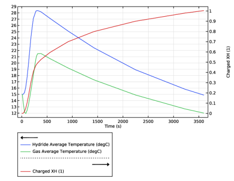
In the Settings window for 1D Plot Group, type Average Temperature and Charged XH in the Label text field.
|
|
1
|
|
2
|
|
3
|
|
4
|
|
5
|
|
1
|
|
2
|
|
3
|
|
1
|
|
2
|
|
3
|
Select the Two y-axes checkbox.
|
|
5
|
|
6
|
|
7
|
|
8
|
|
1
|
|
2
|
|
3
|
|
4
|
Browse to the model’s Application Libraries folder and double-click the file metal_hydride_tank_validation_parameters.txt.
|
|
1
|
In the Model Builder window, under Results > Datasets click Study 1: Cooling Flow/Solution 1 (3) (sol1).
|
|
2
|
|
3
|
|
4
|
|
1
|
|
2
|
|
3
|
|
4
|
|
1
|
|
2
|
|
3
|
|
4
|
|
5
|
|
6
|
|
7
|
Click
|
|
8
|
|
1
|
|
2
|
|
3
|
|
1
|
|
2
|
|
3
|
|
1
|
|
2
|
|
1
|
|
2
|
|
3
|
|
1
|
|
2
|
|
3
|
|
1
|
|
2
|
|
3
|
|
4
|
|
5
|
|
1
|
|
2
|
|
3
|
Clear the Plot dataset edges checkbox.
|
|
4
|
|
5
|
|
6
|
Click
|
|
1
|
|
2
|
|
1
|
|
2
|
|
1
|
|
2
|
|
3
|
|
1
|
|
2
|
|
3
|
|
4
|
|
5
|
|
1
|
|
2
|
|
3
|
|
4
|