PDF

Liquid–Liquid Extraction
Introduction
Liquid–liquid extraction is a process used to separate or transfer species between two immiscible liquids. Transfer of species from one phase to the other is driven by a difference in relative solubility. Often in mixtures consisting of two different phases, one phase disperses within the other phase. This phase is referred to as the dispersed phase, while the other phase is referred to as the continuous phase. Which phase becomes the dispersed phase depends on the density of the two phases.
In this example, a water-filled extraction column is studied. Oil, containing a solute species, is injected at the bottom of the column and rises up due to buoyancy. The raffinate exits at the top of the column. As the oil droplets rise, the solute species is transferred to the solvent, the water phase. Water is initially in the column and is continuously injected at the top. The extract exits at the bottom of the column. In this setup, the water phase becomes the continuous phase and the oil forms droplets as the dispersed phase. The column is fitted with a number of alternating horizontal discs in order to increase the residence time of the oil droplets.
Model Definition
The extraction is modeled using the Dispersed Two-Phase Flow, Diluted Species multiphysics interface, where the k−ω model is used to account for the turbulent flow from the rising droplets. The species transport is solved for in both the continuous (water) phase and in the dispersed phase (oil droplets).
The extraction column can be constructed using a 2D axisymmetric geometry due to rotational symmetry. The column is 0.8 m tall with a radius of 0.1 m. At each end, a wall separates an inflow and outflow. Alternating inner and outer horizontal discs are located throughout the column with a spacing of 0.1 m, as seen in Figure 1. The inner discs have a radius of 0.5 m. The outer disc openings also have a radius of 0.5 m.
Figure 1: Geometry of the modeled extraction column.
Water enters the extraction column at the top inlet and oil enters at the bottom inlet with an oil volume fraction of 0.5. No species is present in the ingoing water. The oil phase enters with a solute species concentration of 10 mol/m3. The water phase at the top inlet has an inlet velocity of 0.01 m/s. The water phase flows from the top to the bottom of the column due to gravity. The density difference between the oil droplets and surrounding water induces buoyancy, causing the droplets to rise through the column.
A pressure condition is used at the outlets. The relative pressure is specified as 0 Pa at the bottom outlet. At the top outlet the relative pressure is specified as
(1)
where g is the gravitational acceleration (m/s2), ρ is the mixture density (kg/m3), and z the height above the column bottom. The flow is solved for by the Mixture Model using the k–ω turbulence model.
Mass transport
The rate of solute extraction, Re (mol/m3/s), from the dispersed phase to the continuous phase is modeled according to
(2)
where km is the mass transfer coefficient (m/s); Kp the partition coefficient; cc and cd the species concentrations in the continuous and dispersed phases (mol/m3), respectively; and as is the specific surface area of the oil droplets per unit volume (1/m). The partition coefficient describes the distribution of solute between the two phases at equilibrium. The specific surface area of the droplets is calculated as
(3)
where the droplets are assumed to be spherical. In this equation, ϕd is the dispersed phase volume fraction and rp is the droplet radius. Including convective and diffusive transport, the time-dependent solute mass transport in the continuous and dispersed phases is modeled according to
(4)
and
(5)
Here, D is the diffusion coefficient (m2/s) and the vector u is the velocity field (m/s). The diffusivity coefficient is the sum of the fluid diffusion and the turbulent diffusion from the multiphysics coupling. The turbulent diffusivity is calculated from the turbulent kinematic viscosity, νt (m2/s) and the turbulent Schmidt number, ScT, as
(6)
To account for the area between the wall and the developed turbulent flow, mass transport wall functions are also modeled using the Dispersed Two-Phase Flow, Diluted Species multiphysics coupling interface.
Results and Discussion
The 2D mixture velocity and phase fluxes at 10 and 210 s is shown in Figure 2. At 10 s the dispersed phase has begun entering the column and the highest mixture velocity can be seen at the oil inlet. At this point the column mainly contains water. The flux of the water phase can be seen from the continuous phase flux streamlines. At 210 s the dispersed phase flux has developed throughout the entire column.
Figure 2: Mixture velocity (m/s) and phase flux stream lines at 10 and 210 s.
The total phase specific solute content is seen in Figure 3. The solute species enters the column with the dispersed phase. As soon as the solute enters the column it begins transferring from the dispersed to the continuous phase. After about 30 s the amount of solute is larger in the continuous phase than in the dispersed phase.
Figure 3: Total amount of solute species in the dispersed and continuous phase.
Figure 4 shows the phase velocities and dispersed phase volume fraction after 210 s. The phase velocities increase when passing through the disc openings as the surface area decreases. The dispersed phase volume fraction is the largest on the bottom of the outer discs.
Figure 4: Phase velocities and dispersed phase volume fraction at 210 s.
The specific phase concentrations and extraction rate is seen in Figure 5. The concentration is overall higher in the dispersed phase than the continuous phase due to the difference in volume. As shown in Equation 2, the extraction rate is the highest where the concentration difference is the largest. This occurs at the bottom of the column, close to the oil inlet.
Figure 5: Phase specific species concentrations and extraction rate at 210 s.
Application Library path: Chemical_Reaction_Engineering_Module/Mixing_and_Separation/liquid_liquid_extraction
Modeling Instructions
From the File menu, choose New.
New
In the New window, click  Model Wizard.
Model Wizard
1
In the Model Wizard window, click  2D Axisymmetric.
2
In the Select Physics tree, select Chemical Species Transport > Dispersed Two-Phase Flow with Species Transport > Turbulent Flow > Turbulent Flow, k-ω.
3
Click Add.
4
In the Added physics interfaces tree, select Continuous Phase Transport of Diluted Species (tds).
5
In the Concentrations (mol/m³) table, enter the following settings:
6
In the Added physics interfaces tree, select Dispersed Phase Transport of Diluted Species (tds2).
7
In the Concentrations (mol/m³) table, enter the following settings:
8
Click  Study.
9
In the Select Study tree, select General Studies > Time Dependent.
10
Import the parameters for the model.
Global Definitions
Parameters 1
1
In the Model Builder window, under Global Definitions click Parameters 1.
2
In the Settings window for Parameters, locate the Parameters section.
3
Click  Load from File.
4
Definitions
Define step functions that will be used to smoothen sharp transitions in the model.
Step 1 (step1)
1
In the Definitions toolbar, click  More Functions and choose Step.
2
In the Settings window for Step, locate the Parameters section.
3
In the Location text field, type 0.64.
4
In the From text field, type 1.
5
In the To text field, type 0.
6
Click to expand the Smoothing section. In the Size of transition zone text field, type 0.15.
Step 2 (step2)
1
In the Definitions toolbar, click  More Functions and choose Step.
2
In the Settings window for Step, locate the Parameters section.
3
In the Location text field, type 0.5.
4
Locate the Smoothing section. In the Size of transition zone text field, type 1[s].
Step 3 (step3)
1
In the Definitions toolbar, click  More Functions and choose Step.
2
In the Settings window for Step, locate the Parameters section.
3
In the Location text field, type 2.25.
4
Locate the Smoothing section. In the Size of transition zone text field, type 0.5[s].
Geometry 1
Rectangle 1 (r1)
1
In the Geometry toolbar, click  Rectangle.
2
In the Settings window for Rectangle, locate the Size and Shape section.
3
In the Width text field, type R_c.
4
In the Height text field, type H_c.
5
Click to expand the Layers section. In the table, enter the following settings:
6
Select the Layers to the right checkbox.
7
Clear the Layers on bottom checkbox.
Rectangle 2 (r2)
1
In the Geometry toolbar, click  Rectangle.
2
In the Settings window for Rectangle, locate the Size and Shape section.
3
In the Width text field, type W_sep.
4
In the Height text field, type H_sep.
5
Locate the Position section. In the r text field, type R_c*0.4.
Mirror the geometry to cover the entire extraction column.
Mirror 1 (mir1)
1
In the Geometry toolbar, click  Transforms and choose Mirror.
2
3
In the Settings window for Mirror, locate the Input section.
4
Select the Keep input objects checkbox.
5
Locate the Point on Line of Reflection section. In the z text field, type H_c/2.
6
Locate the Normal Vector to Line of Reflection section. In the r text field, type 0.
7
In the z text field, type 1.
Polygon 1 (pol1)
1
In the Geometry toolbar, click  Polygon.
2
In the Settings window for Polygon, locate the Coordinates section.
3
Array 1 (arr1)
1
In the Geometry toolbar, click  Transforms and choose Array.
2
3
In the Settings window for Array, locate the Size section.
4
In the z size text field, type n_s.
5
Locate the Displacement section. In the z text field, type hsep_s*2.
Mirror 2 (mir2)
1
In the Geometry toolbar, click  Transforms and choose Mirror.
2
Select the objects arr1(1,1), arr1(1,2), and arr1(1,3) only.
3
In the Settings window for Mirror, locate the Input section.
4
Select the Keep input objects checkbox.
5
Locate the Point on Line of Reflection section. In the r text field, type (R_c-t_c)/2.
Move 1 (mov1)
1
In the Geometry toolbar, click  Transforms and choose Move.
2
Select the objects mir2(1), mir2(2), and mir2(3) only.
3
In the Settings window for Move, locate the Displacement section.
4
In the z text field, type hsep_s.
Rectangle 3 (r3)
1
In the Geometry toolbar, click  Rectangle.
2
In the Settings window for Rectangle, locate the Size and Shape section.
3
In the Width text field, type R_c*0.4*0.9.
4
In the Height text field, type h0_s*0.85.
Mesh Control Domains 1 (mcd1)
1
In the Geometry toolbar, click  Virtual Operations and choose Mesh Control Domains.
2
On the object fin, select Domain 1 only.
3
In the Geometry toolbar, click  Build All.
Definitions
Column interior
1
In the Definitions toolbar, click  Explicit.
2
In the Settings window for Explicit, type Column interior in the Label text field.
3
Maximum 1 (maxop1)
1
In the Definitions toolbar, click  Nonlocal Couplings and choose Maximum.
2
Minimum 1 (minop1)
1
In the Definitions toolbar, click  Nonlocal Couplings and choose Minimum.
2
In the Settings window for Minimum, locate the Source Selection section.
3
From the Selection list, choose All domains.
Add Material
1
In the Home toolbar, click  Add Material to open the Add Material window.
2
Go to the Add Material window.
3
In the tree, select Built-in > Water, liquid.
4
Click the Add to Component button in the window toolbar.
5
In the Home toolbar, click  Add Material to close the Add Material window.
Mixture Model, k-ω (mm)
1
In the Settings window for Mixture Model, k-ω, locate the Domain Selection section.
2
From the Selection list, choose Column interior.
3
Locate the Physical Model section. From the Dispersed phase list, choose Liquid droplets/bubbles.
4
From the Slip model list, choose Schiller–Naumann.
Mixture Properties 1
1
In the Model Builder window, under Component 1 (comp1) > Mixture Model, k-ω (mm) click Mixture Properties 1.
2
In the Settings window for Mixture Properties, locate the Materials section.
3
From the Dispersed phase list, choose Domain material.
4
Locate the Dispersed Phase Properties section. From the ρd list, choose User defined. In the associated text field, type rho_d.
5
From the μd list, choose User defined. In the associated text field, type mu_d.
6
In the dd text field, type 2*r_d.
7
Locate the Mixture Model section. From the Mixture viscosity model list, choose Volume averaged.
Gravity 1
1
In the Physics toolbar, click  Domains and choose Gravity.
2
Outlet 1
1
In the Physics toolbar, click  Boundaries and choose Outlet.
2
3
In the Settings window for Outlet, locate the Pressure section.
4
Clear the Suppress backflow checkbox.
5
Locate the Dispersed Phase Boundary Condition section. Select the Exterior dispersed phase conditions checkbox.
6
In the ϕd,0 text field, type 1e-6.
Outlet 2
1
In the Physics toolbar, click  Boundaries and choose Outlet.
2
3
In the Settings window for Outlet, locate the Pressure section.
4
In the p0 text field, type -g_const*mm.rho*z.
5
Locate the Dispersed Phase Boundary Condition section. Select the Exterior dispersed phase conditions checkbox.
6
In the ϕd,0 text field, type 1e-6.
Inlet 1
1
In the Physics toolbar, click  Boundaries and choose Inlet.
2
3
In the Settings window for Inlet, locate the Velocity section.
4
In the J0 text field, type nojac(mm.jslipz).
5
Locate the Dispersed Phase Boundary Condition section. In the ϕd,0 text field, type vf0*step2(t).
Inlet 2
1
In the Physics toolbar, click  Boundaries and choose Inlet.
2
3
In the Settings window for Inlet, locate the Velocity section.
4
In the J0 text field, type 0.01[m/s]*step2(t).
Continuous Phase Transport of Diluted Species (tds)
1
In the Model Builder window, under Component 1 (comp1) click Continuous Phase Transport of Diluted Species (tds).
2
In the Settings window for Continuous Phase Transport of Diluted Species, locate the Domain Selection section.
3
From the Selection list, choose Column interior.
Fluid 1
1
In the Model Builder window, under Component 1 (comp1) > Continuous Phase Transport of Diluted Species (tds) click Fluid 1.
2
In the Settings window for Fluid, locate the Diffusion section.
3
In the Dcc text field, type D1.
Inflow 1
1
In the Physics toolbar, click  Boundaries and choose Inflow.
2
Open Boundary 1
1
In the Physics toolbar, click  Boundaries and choose Open Boundary.
2
3
In the Settings window for Open Boundary, locate the Exterior Concentration section.
4
In the c0,cc text field, type 1e-6.
Dispersed Phase Transport of Diluted Species 2 (tds2)
1
In the Model Builder window, under Component 1 (comp1) click Dispersed Phase Transport of Diluted Species 2 (tds2).
2
In the Settings window for Dispersed Phase Transport of Diluted Species, locate the Domain Selection section.
3
From the Selection list, choose Column interior.
Fluid 1
1
In the Model Builder window, under Component 1 (comp1) > Dispersed Phase Transport of Diluted Species 2 (tds2) click Fluid 1.
2
In the Settings window for Fluid, locate the Diffusion section.
3
In the Dcd text field, type D1.
Inflow 1
1
In the Physics toolbar, click  Boundaries and choose Inflow.
2
3
In the Settings window for Inflow, locate the Concentration section.
4
In the c0,cd text field, type cd_0*vf0*step3(t).
Open Boundary 1
1
In the Physics toolbar, click  Boundaries and choose Open Boundary.
2
3
In the Settings window for Open Boundary, locate the Exterior Concentration section.
4
In the c0,cd text field, type 1e-6.
Multiphysics
Dispersed Two-Phase Flow, Diluted Species 1 (dds1)
1
In the Model Builder window, under Component 1 (comp1) > Multiphysics click Dispersed Two-Phase Flow, Diluted Species 1 (dds1).
2
In the Settings window for Dispersed Two-Phase Flow, Diluted Species, locate the Solute Extraction section.
3
Select the Species cc checkbox.
4
In the km,cc text field, type km*step1(phid).
5
In the Kp,cc text field, type K_p.
Mesh 1
1
In the Model Builder window, under Component 1 (comp1) click Mesh 1.
2
In the Settings window for Mesh, locate the Sequence Type section.
3
From the list, choose User-controlled mesh.
Size
1
In the Model Builder window, under Component 1 (comp1) > Mesh 1 click Size.
2
In the Settings window for Size, locate the Element Size section.
3
From the Predefined list, choose Coarse.
4
Click the Custom button.
5
Locate the Element Size Parameters section. In the Maximum element size text field, type 0.005.
6
In the Minimum element size text field, type 4.0E-5.
7
In the Curvature factor text field, type 0.25.
Corner Refinement 1
1
In the Model Builder window, click Corner Refinement 1.
2
In the Settings window for Corner Refinement, locate the Angle section.
3
In the Minimum angle between boundaries text field, type 200.
4
Locate the Refinement section. In the Element size scaling factor text field, type 0.2.
Free Triangular 1
1
In the Model Builder window, click Free Triangular 1.
2
In the Settings window for Free Triangular, locate the Domain Selection section.
3
From the Geometric entity level list, choose Remaining.
Boundary Layers 1
1
In the Model Builder window, click Boundary Layers 1.
2
In the Settings window for Boundary Layers, click to expand the Corner Settings section.
3
From the Handling of sharp corners list, choose Splitting.
4
In the Maximum angle per split text field, type 45.
5
Click to expand the Transition section. In the Number of iterations text field, type 10.
Size 2
1
In the Mesh toolbar, click  Sizing and choose Size.
2
In the Settings window for Size, locate the Geometric Entity Selection section.
3
From the Geometric entity level list, choose Domain.
4
5
Locate the Element Size section. From the Calibrate for list, choose Fluid dynamics.
6
From the Predefined list, choose Finer.
7
8
Click  Build All.
Study 1
1
In the Model Builder window, click Study 1.
2
In the Settings window for Study, locate the Study Settings section.
3
Clear the Generate default plots checkbox.
Change the time interval to see the startup process.
Step 1: Time Dependent
1
In the Model Builder window, under Study 1 click Step 1: Time Dependent.
2
In the Settings window for Time Dependent, locate the Study Settings section.
3
In the Output times text field, type range(0,1,210).
Solution 1 (sol1)
1
In the Study toolbar, click  Show Default Solver.
2
In the Model Builder window, expand the Solution 1 (sol1) node.
3
In the Model Builder window, expand the Study 1 > Solver Configurations > Solution 1 (sol1) > Dependent Variables 1 node, then click Concentration (comp1.cc).
4
In the Settings window for Field, locate the Scaling section.
5
From the Method list, choose Manual.
6
In the Model Builder window, under Study 1 > Solver Configurations > Solution 1 (sol1) > Dependent Variables 1 click Concentration (comp1.cd).
7
In the Settings window for Field, locate the Scaling section.
8
From the Method list, choose Manual.
9
In the Model Builder window, under Study 1 > Solver Configurations > Solution 1 (sol1) > Dependent Variables 1 click Wall Concentration, Downside (comp1.dds1.cWall_d_cc).
10
In the Settings window for Field, locate the Scaling section.
11
From the Method list, choose Manual.
12
In the Model Builder window, under Study 1 > Solver Configurations > Solution 1 (sol1) > Dependent Variables 1 click Wall Concentration, Downside (comp1.dds1.cWall_d_cd).
13
In the Settings window for Field, locate the Scaling section.
14
From the Method list, choose Manual.
15
In the Model Builder window, under Study 1 > Solver Configurations > Solution 1 (sol1) > Dependent Variables 1 click Wall Concentration, Upside (comp1.dds1.cWall_u_cc).
16
In the Settings window for Field, locate the Scaling section.
17
From the Method list, choose Manual.
18
In the Model Builder window, under Study 1 > Solver Configurations > Solution 1 (sol1) > Dependent Variables 1 click Wall Concentration, Upside (comp1.dds1.cWall_u_cd).
19
In the Settings window for Field, locate the Scaling section.
20
From the Method list, choose Manual.
21
In the Model Builder window, under Study 1 > Solver Configurations > Solution 1 (sol1) > Dependent Variables 1 click Velocity Field, Mixture (comp1.j).
22
In the Settings window for Field, locate the Scaling section.
23
From the Method list, choose Manual.
24
In the Scale text field, type 0.1.
25
In the Model Builder window, under Study 1 > Solver Configurations > Solution 1 (sol1) > Dependent Variables 1 click Pressure (comp1.p).
26
In the Settings window for Field, locate the Scaling section.
27
From the Method list, choose Manual.
28
In the Scale text field, type 1e4.
Modify the maximum step constraint.
29
In the Model Builder window, under Study 1 > Solver Configurations > Solution 1 (sol1) click Time-Dependent Solver 1.
30
In the Settings window for Time-Dependent Solver, click to expand the Time Stepping section.
31
From the Maximum step constraint list, choose Constant.
32
In the Maximum step text field, type 5e-3.
33
In the Study toolbar, click  Compute.
Results
Revolution 2D 1
1
In the Model Builder window, expand the Results node.
2
Right-click Results > Datasets and choose Revolution 2D.
3
In the Settings window for Revolution 2D, click to expand the Revolution Layers section.
4
In the Revolution angle text field, type 180.
Revolution 2D 2
In the Results toolbar, click  More Datasets and choose Revolution 2D.
Selection
1
In the Results toolbar, click  Attributes and choose Selection.
2
In the Settings window for Selection, locate the Geometric Entity Selection section.
3
From the Geometric entity level list, choose Domain.
4
Revolution 2D 3
1
In the Results toolbar, click  More Datasets and choose Revolution 2D.
2
In the Settings window for Revolution 2D, locate the Revolution Layers section.
3
In the Revolution angle text field, type 225.
Selection
1
In the Results toolbar, click  Attributes and choose Selection.
2
In the Settings window for Selection, locate the Geometric Entity Selection section.
3
From the Geometric entity level list, choose Domain.
4
Cut Plane 1
1
In the Results toolbar, click  Cut Plane.
2
In the Settings window for Cut Plane, locate the Plane Data section.
3
From the Plane list, choose xz-planes.
Now, show the mixture velocity and the phase fluxes with streamlines.
Mixture Velocity and Phase Flux Streamlines
1
In the Results toolbar, click  2D Plot Group.
2
In the Settings window for 2D Plot Group, type Mixture Velocity and Phase Flux Streamlines in the Label text field.
3
Click to expand the Title section. From the Title type list, choose None.
4
Click to expand the Color Legend section. Select the Show units checkbox.
5
Click to expand the Plot Array section. From the Array type list, choose Linear.
6
In the Relative padding text field, type 0.5.
Mixture Velocity
1
In the Mixture Velocity and Phase Flux Streamlines toolbar, click  Surface.
2
In the Settings window for Surface, type Mixture Velocity in the Label text field.
3
Locate the Data section. From the Dataset list, choose Study 1/Solution 1 (sol1).
4
From the Time (s) list, choose 10.
5
Click Replace Expression in the upper-right corner of the Expression section. From the menu, choose Component 1 (comp1) > Mixture Model, k-ω > Velocity and pressure > mm.J - Velocity field, mixture - m/s.
Mixture Velocity and Phase Flux Streamlines
In the Mixture Velocity and Phase Flux Streamlines toolbar, click  Streamline.
Phase Flux, Dispersed Phase
1
In the Settings window for Streamline, type Phase Flux, Dispersed Phase in the Label text field.
2
Locate the Data section. From the Dataset list, choose Study 1/Solution 1 (sol1).
3
From the Time (s) list, choose 10.
4
Click Replace Expression in the upper-right corner of the Expression section. From the menu, choose Component 1 (comp1) > Mixture Model, k-ω > Fluxes > mm.jdr,mm.jdz - Dispersed phase flux.
5
Locate the Streamline Positioning section. From the Positioning list, choose Uniform density.
6
In the Density level text field, type 7.8.
7
Locate the Coloring and Style section. Find the Point style subsection. From the Type list, choose Arrow.
Phase Flux, Continuous Phase
1
Right-click Phase Flux, Dispersed Phase and choose Duplicate.
2
In the Settings window for Streamline, type Phase Flux, Continuous Phase in the Label text field.
3
Click Replace Expression in the upper-right corner of the Expression section. From the menu, choose Component 1 (comp1) > Mixture Model, k-ω > Fluxes > mm.jcr,mm.jcz - Continuous phase flux.
Mixture Velocity and Phase Flux Streamlines
In the Mixture Velocity and Phase Flux Streamlines toolbar, click  Annotation.
Annotation 1
1
In the Settings window for Annotation, locate the Annotation section.
2
In the Text text field, type Time = 10 s, Mixture Velocity.
3
Locate the Position section. In the r text field, type -0.035.
4
Locate the Coloring and Style section. Clear the Show point checkbox.
5
From the Orientation list, choose Vertical.
6
Click to expand the Plot Array section. Select the Manual indexing checkbox.
Annotation 2
1
Right-click Results > Mixture Velocity and Phase Flux Streamlines > Annotation 1 and choose Duplicate.
2
In the Settings window for Annotation, locate the Annotation section.
3
In the Text text field, type Time = 10 s, Dispersed Phase Flux.
4
Locate the Plot Array section. In the Index text field, type 1.
Annotation 3
1
Right-click Annotation 2 and choose Duplicate.
2
In the Settings window for Annotation, locate the Annotation section.
3
In the Text text field, type Time = 10 s, Continuous Phase Flux.
4
Locate the Plot Array section. In the Index text field, type 2.
Annotation 1, Annotation 2, Annotation 3, Mixture Velocity, Phase Flux, Continuous Phase, Phase Flux, Dispersed Phase
1
In the Model Builder window, under Results > Mixture Velocity and Phase Flux Streamlines, Ctrl-click to select Mixture Velocity, Phase Flux, Dispersed Phase, Phase Flux, Continuous Phase, Annotation 1, Annotation 2, and Annotation 3.
2
Mixture Velocity 1
1
In the Settings window for Surface, locate the Data section.
2
From the Time (s) list, choose 210.
3
Click to expand the Inherit Style section. From the Plot list, choose Mixture Velocity.
Phase Flux, Dispersed Phase 1
1
In the Model Builder window, click Phase Flux, Dispersed Phase 1.
2
In the Settings window for Streamline, locate the Data section.
3
From the Time (s) list, choose 210.
Phase Flux, Continuous Phase 1
1
In the Model Builder window, click Phase Flux, Continuous Phase 1.
2
In the Settings window for Streamline, locate the Data section.
3
From the Time (s) list, choose 210.
Annotation 4
1
In the Model Builder window, click Annotation 4.
2
In the Settings window for Annotation, locate the Annotation section.
3
In the Text text field, type Time = 210 s, Mixture Velocity.
4
Locate the Plot Array section. In the Index text field, type 3.
Annotation 5
1
In the Model Builder window, click Annotation 5.
2
In the Settings window for Annotation, locate the Annotation section.
3
In the Text text field, type Time = 210 s, Dispersed Phase Flux.
4
Locate the Plot Array section. In the Index text field, type 4.
Annotation 6
1
In the Model Builder window, click Annotation 6.
2
In the Settings window for Annotation, locate the Annotation section.
3
In the Text text field, type Time = 210 s, Continuous Phase Flux.
4
Locate the Plot Array section. In the Index text field, type 5.
5
In the Mixture Velocity and Phase Flux Streamlines toolbar, click  Plot.
6
Click the  Show Grid button in the Graphics toolbar.
7
Click the  Zoom Extents button in the Graphics toolbar.
Next, create a plot to show the phase velocities and dispersed phase volume fraction in 3D.
Phase Velocities and Volume Fraction (3D)
1
In the Results toolbar, click  3D Plot Group.
2
In the Settings window for 3D Plot Group, type Phase Velocities and Volume Fraction (3D) in the Label text field.
3
Click to expand the Title section. From the Title type list, choose None.
4
Locate the Plot Settings section. Clear the Plot dataset edges checkbox.
5
Locate the Color Legend section. Select the Show units checkbox.
6
Click to expand the Plot Array section. From the Array type list, choose Linear.
7
From the Padding list, choose Absolute.
8
In the Padding length text field, type 0.2.
Stages
1
In the Phase Velocities and Volume Fraction (3D) toolbar, click  Surface.
2
In the Settings window for Surface, type Stages in the Label text field.
3
Locate the Data section. From the Dataset list, choose Revolution 2D 2.
4
Locate the Expression section. In the Expression text field, type 1.
5
Click to expand the Plot Array section. Select the Manual indexing checkbox.
Material Appearance 1
1
In the Phase Velocities and Volume Fraction (3D) toolbar, click  Material Appearance.
2
In the Settings window for Material Appearance, locate the Appearance section.
3
From the Appearance list, choose Custom.
4
From the Material type list, choose Steel (anodized).
Column
1
In the Model Builder window, right-click Stages and choose Duplicate.
2
In the Settings window for Surface, type Column in the Label text field.
3
Locate the Data section. From the Dataset list, choose Revolution 2D 3.
Phase Velocities and Volume Fraction (3D)
In the Phase Velocities and Volume Fraction (3D) toolbar, click  Surface.
Velocity, Dispersed Phase
1
In the Settings window for Surface, type Velocity, Dispersed Phase in the Label text field.
2
Click Replace Expression in the upper-right corner of the Expression section. From the menu, choose Component 1 (comp1) > Mixture Model, k-ω > Velocity and pressure > mm.Ud - Velocity field, dispersed phase - m/s.
3
Locate the Plot Array section. Select the Manual indexing checkbox.
Phase Velocities and Volume Fraction (3D)
In the Phase Velocities and Volume Fraction (3D) toolbar, click  More Plots and choose Streamline Surface.
Velocity Field, Dispersed Phase
1
In the Settings window for Streamline Surface, type Velocity Field, Dispersed Phase in the Label text field.
2
Locate the Data section. From the Dataset list, choose Cut Plane 1.
3
Click Replace Expression in the upper-right corner of the Expression section. From the menu, choose Component 1 (comp1) > Mixture Model, k-ω > Velocity and pressure > mm.udr,...,mm.udz - Velocity field, dispersed phase.
4
Locate the Streamline Positioning section. From the Positioning list, choose Uniform density.
5
In the Density level text field, type 8.5.
6
Locate the Coloring and Style section. Find the Line style subsection. From the Type list, choose Tube.
7
Select the Radius scale factor checkbox. In the associated text field, type 0.0015.
8
Find the Point style subsection. From the Type list, choose Arrow.
9
Select the Scale factor checkbox. In the associated text field, type 0.2.
10
From the Color list, choose Custom.
11
12
Click Define custom colors.
13
14
Click Add to custom colors.
15
Click Show color palette only or OK on the cross-platform desktop.
16
Click to expand the Plot Array section. Select the Manual indexing checkbox.
Phase Velocities and Volume Fraction (3D)
In the Phase Velocities and Volume Fraction (3D) toolbar, click  Annotation.
Annotation 1
1
In the Settings window for Annotation, locate the Annotation section.
2
In the Text text field, type Dispersed Phase Velocity.
3
Locate the Position section. In the x text field, type 1.5*R_c.
4
In the z text field, type H_c/2.
5
Locate the Coloring and Style section. Clear the Show point checkbox.
6
From the Anchor point list, choose Center.
7
From the Orientation list, choose Vertical.
Annotation 1, Column, Stages, Velocity Field, Dispersed Phase, Velocity, Dispersed Phase
1
In the Model Builder window, under Results > Phase Velocities and Volume Fraction (3D), Ctrl-click to select Stages, Column, Velocity, Dispersed Phase, Velocity Field, Dispersed Phase, and Annotation 1.
2
Stages 1
1
In the Settings window for Surface, locate the Plot Array section.
2
In the Index text field, type 1.
Column 1
1
In the Model Builder window, click Column 1.
2
In the Settings window for Surface, locate the Plot Array section.
3
In the Index text field, type 1.
Velocity, Continuous Phase
1
In the Model Builder window, under Results > Phase Velocities and Volume Fraction (3D) click Velocity, Dispersed Phase 1.
2
In the Settings window for Surface, type Velocity, Continuous Phase in the Label text field.
3
Click Replace Expression in the upper-right corner of the Expression section. From the menu, choose Component 1 (comp1) > Mixture Model, k-ω > Velocity and pressure > mm.Uc - Velocity field, continuous phase - m/s.
4
Click to expand the Inherit Style section. From the Plot list, choose Velocity, Dispersed Phase.
5
Locate the Plot Array section. In the Index text field, type 1.
Velocity Field, Continuous Phase
1
In the Model Builder window, under Results > Phase Velocities and Volume Fraction (3D) click Velocity Field, Dispersed Phase 1.
2
In the Settings window for Streamline Surface, type Velocity Field, Continuous Phase in the Label text field.
3
Click Replace Expression in the upper-right corner of the Expression section. From the menu, choose Component 1 (comp1) > Mixture Model, k-ω > Velocity and pressure > mm.ucr,...,mm.ucz - Velocity field, continuous phase.
4
Locate the Plot Array section. In the Index text field, type 1.
Annotation 2
1
In the Model Builder window, click Annotation 2.
2
In the Settings window for Annotation, locate the Annotation section.
3
In the Text text field, type Continuous Phase Velocity.
Annotation 1, Column, Stages, Velocity, Dispersed Phase
1
In the Model Builder window, under Results > Phase Velocities and Volume Fraction (3D), Ctrl-click to select Stages, Column, Velocity, Dispersed Phase, and Annotation 1.
2
Stages 2
1
In the Settings window for Surface, locate the Plot Array section.
2
In the Index text field, type 2.
Column 2
1
In the Model Builder window, click Column 2.
2
In the Settings window for Surface, locate the Plot Array section.
3
In the Index text field, type 2.
Volume Fraction, Dispersed Phase
1
In the Model Builder window, under Results > Phase Velocities and Volume Fraction (3D) click Velocity, Dispersed Phase 1.
2
In the Settings window for Surface, type Volume Fraction, Dispersed Phase in the Label text field.
3
Click Replace Expression in the upper-right corner of the Expression section. From the menu, choose Component 1 (comp1) > Mixture Model, k-ω > mm.phidReg - Volume fraction, dispersed phase - 1.
4
Locate the Coloring and Style section. From the Color table list, choose AuroraBorealis.
5
Locate the Plot Array section. In the Index text field, type 2.
Annotation 3
1
In the Model Builder window, click Annotation 3.
2
In the Settings window for Annotation, locate the Annotation section.
3
In the Text text field, type Dispersed Phase Volume Fraction.
4
In the Phase Velocities and Volume Fraction (3D) toolbar, click  Plot.
5
Click the  Zoom Extents button in the Graphics toolbar.
Create a second 3D plot group to show the phase concentrations and the solute extraction rate.
Phase Concentrations and Solute Extraction Rate (3D)
1
In the Model Builder window, right-click Phase Velocities and Volume Fraction (3D) and choose Duplicate.
2
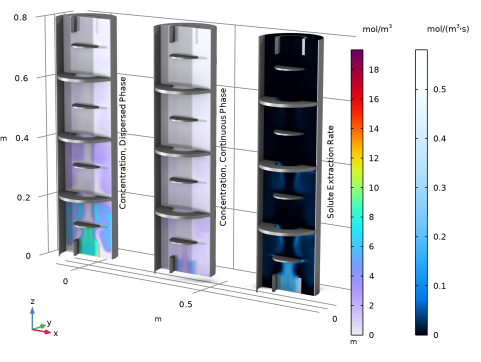
In the Settings window for 3D Plot Group, type Phase Concentrations and Solute Extraction Rate (3D) in the Label text field.
3
In the Model Builder window, expand the Phase Concentrations and Solute Extraction Rate (3D) node.
Velocity Field, Continuous Phase, Velocity Field, Dispersed Phase
1
In the Model Builder window, under Results > Phase Concentrations and Solute Extraction Rate (3D), Ctrl-click to select Velocity Field, Dispersed Phase and Velocity Field, Continuous Phase.
2
Concentration, Dispersed Phase
1
In the Model Builder window, under Results > Phase Concentrations and Solute Extraction Rate (3D) click Velocity, Dispersed Phase.
2
In the Settings window for Surface, type Concentration, Dispersed Phase in the Label text field.
3
Click Replace Expression in the upper-right corner of the Expression section. From the menu, choose Component 1 (comp1) > Dispersed Phase Transport of Diluted Species 2 > Species cd > tds2.phs_cd - Phase specific concentration - mol/m³.
4
Locate the Coloring and Style section. From the Color table list, choose Prism.
Annotation 1
1
In the Model Builder window, click Annotation 1.
2
In the Settings window for Annotation, locate the Annotation section.
3
In the Text text field, type Concentration, Dispersed Phase.
Concentration, Continuous Phase
1
In the Model Builder window, under Results > Phase Concentrations and Solute Extraction Rate (3D) click Velocity, Continuous Phase.
2
In the Settings window for Surface, type Concentration, Continuous Phase in the Label text field.
3
Click Replace Expression in the upper-right corner of the Expression section. From the menu, choose Component 1 (comp1) > Continuous Phase Transport of Diluted Species > Species cc > tds.phs_cc - Phase specific concentration - mol/m³.
Annotation 2
1
In the Model Builder window, click Annotation 2.
2
In the Settings window for Annotation, locate the Annotation section.
3
In the Text text field, type Concentration, Continuous Phase.
Solute Extraction Rate
1
In the Model Builder window, under Results > Phase Concentrations and Solute Extraction Rate (3D) click Volume Fraction, Dispersed Phase.
2
In the Settings window for Surface, type Solute Extraction Rate in the Label text field.
3
Locate the Expression section. In the Expression text field, type dds1.Re_cc.
4
Locate the Coloring and Style section. From the Color table list, choose JupiterAuroraBorealis.
Annotation 3
1
In the Model Builder window, click Annotation 3.
2
In the Settings window for Annotation, locate the Annotation section.
3
In the Text text field, type Solute Extraction Rate.
4
In the Phase Concentrations and Solute Extraction Rate (3D) toolbar, click  Plot.
Create a plot to show the column geometry in 3D.
Geometry
1
In the Results toolbar, click  3D Plot Group.
2
In the Settings window for 3D Plot Group, type Geometry in the Label text field.
3
Locate the Title section. From the Title type list, choose None.
4
Locate the Plot Settings section. Clear the Plot dataset edges checkbox.
Stages
1
In the Geometry toolbar, click  Surface.
2
In the Settings window for Surface, locate the Expression section.
3
In the Expression text field, type 1.
4
Locate the Data section. From the Dataset list, choose Revolution 2D 2.
5
In the Label text field, type Stages.
Material Appearance 1
1
In the Geometry toolbar, click  Material Appearance.
2
In the Settings window for Material Appearance, locate the Appearance section.
3
From the Appearance list, choose Custom.
4
From the Material type list, choose Steel (anodized).
Column
1
In the Model Builder window, right-click Stages and choose Duplicate.
2
In the Settings window for Surface, locate the Data section.
3
From the Dataset list, choose Revolution 2D 3.
4
In the Label text field, type Column.
5
In the Geometry toolbar, click  Plot.
Next, create a set of 1D plots to show the total phase concentrations and boundary fluxes.
Evaluation Group 1
In the Results toolbar, click  Evaluation Group.
Surface Integration 1
1
In the Evaluation Group 1 toolbar, click  Integration and choose Surface Integration.
2
In the Settings window for Surface Integration, locate the Selection section.
3
From the Selection list, choose Column interior.
4
Locate the Expressions section. In the table, enter the following settings:
Evaluate the expressions and plot them in a table graph.
5
In the Evaluation Group 1 toolbar, click  Evaluate.
1D Plot Group 5
In the Evaluation Group 1 toolbar, click  Table Graph.
Table Graph 1
1
In the Settings window for Table Graph, click to expand the Coloring and Style section.
2
From the Width list, choose 2.
3
Click to expand the Legends section. Select the Show legends checkbox.
4
From the Legends list, choose Manual.
5
1D Plot Group 5
1
In the Model Builder window, click 1D Plot Group 5.
2
In the Settings window for 1D Plot Group, click to expand the Plot Settings section.
3
Select the y-axis label checkbox. In the associated text field, type Amount (mol).
4
Locate the Legend section. From the Position list, choose Upper left.
Evaluation Group 2
In the Results toolbar, click  Evaluation Group.
Line Integration 1
1
In the Evaluation Group 2 toolbar, click  Integration and choose Line Integration.
2
3
In the Settings window for Line Integration, locate the Expressions section.
4
Evaluation Group 2
In the Evaluation Group 2 toolbar, click  Integration and choose Line Integration.
Line Integration 2
1
2
In the Settings window for Line Integration, locate the Expressions section.
3
Evaluation Group 2
In the Evaluation Group 2 toolbar, click  Integration and choose Line Integration.
Line Integration 3
1
2
In the Settings window for Line Integration, locate the Expressions section.
3
Evaluation Group 2
In the Evaluation Group 2 toolbar, click  Integration and choose Line Integration.
Line Integration 4
1
2
In the Settings window for Line Integration, locate the Expressions section.
3
4
In the Evaluation Group 2 toolbar, click  Evaluate.
1D Plot Group 6
In the Evaluation Group 2 toolbar, click  Table Graph.
Table Graph 1
1
In the Settings window for Table Graph, locate the Legends section.
2
Select the Show legends checkbox.
1D Plot Group 6
1
In the Model Builder window, click 1D Plot Group 6.
2
In the Settings window for 1D Plot Group, locate the Legend section.
3
From the Position list, choose Upper left.
Evaluation Group 3
In the Model Builder window, under Results right-click Evaluation Group 2 and choose Duplicate.
Line Integration 1
1
In the Model Builder window, expand the Evaluation Group 3 node, then click Line Integration 1.
2
In the Settings window for Line Integration, locate the Expressions section.
3
Line Integration 2
1
In the Model Builder window, click Line Integration 2.
2
In the Settings window for Line Integration, locate the Expressions section.
3
Line Integration 3
1
In the Model Builder window, click Line Integration 3.
2
In the Settings window for Line Integration, locate the Expressions section.
3
Line Integration 4
1
In the Model Builder window, click Line Integration 4.
2
In the Settings window for Line Integration, locate the Expressions section.
3
4
In the Evaluation Group 3 toolbar, click  Evaluate.
1D Plot Group 7
In the Evaluation Group 3 toolbar, click  Table Graph.
Table Graph 1
1
In the Settings window for Table Graph, locate the Legends section.
2
Select the Show legends checkbox.
1D Plot Group 7
1
In the Model Builder window, click 1D Plot Group 7.
2
In the Settings window for 1D Plot Group, locate the Legend section.
3
From the Position list, choose Upper left.
Evaluation Group 4
In the Results toolbar, click  Evaluation Group.
Line Integration 1
1
In the Evaluation Group 4 toolbar, click  Integration and choose Line Integration.
2
3
In the Settings window for Line Integration, locate the Expressions section.
4
5
Locate the Data Series Operation section. From the Transformation list, choose Integral.
6
Select the Cumulative checkbox.
Evaluation Group 4
In the Evaluation Group 4 toolbar, click  Integration and choose Line Integration.
Line Integration 2
1
2
In the Settings window for Line Integration, locate the Expressions section.
3
4
Locate the Data Series Operation section. From the Transformation list, choose Integral.
5
Select the Cumulative checkbox.
6
In the Evaluation Group 4 toolbar, click  Evaluate.
1D Plot Group 8
In the Evaluation Group 4 toolbar, click  Table Graph.
Table Graph 1
1
In the Settings window for Table Graph, click to expand the Coloring and Style section.
2
From the Width list, choose 2.
3
Locate the Legends section. Select the Show legends checkbox.
4
From the Legends list, choose Manual.
5
1D Plot Group 8
1
In the Model Builder window, click 1D Plot Group 8.
2
In the Settings window for 1D Plot Group, locate the Plot Settings section.
3
Select the y-axis label checkbox. In the associated text field, type Amount (mol).
4
Locate the Legend section. From the Position list, choose Upper left.
5
In the 1D Plot Group 8 toolbar, click  Plot.
1D Plot Group 5, Evaluation Group 1
1
In the Model Builder window, under Results, Ctrl-click to select 1D Plot Group 5 and Evaluation Group 1.
2
Phase Concentrations
In the Settings window for Group, type Phase Concentrations in the Label text field.
1D Plot Group 6, Evaluation Group 2
1
In the Model Builder window, under Results, Ctrl-click to select 1D Plot Group 6 and Evaluation Group 2.
2
Boundary Fluxes, Dispersed Phase
In the Settings window for Group, type Boundary Fluxes, Dispersed Phase in the Label text field.
1D Plot Group 7, Evaluation Group 3
1
In the Model Builder window, under Results, Ctrl-click to select 1D Plot Group 7 and Evaluation Group 3.
2
Boundary Fluxes, Continuous Phase
In the Settings window for Group, type Boundary Fluxes, Continuous Phase in the Label text field.
1D Plot Group 8, Evaluation Group 4
1
In the Model Builder window, under Results, Ctrl-click to select 1D Plot Group 8 and Evaluation Group 4.
2
Species Boundary Fluxes
In the Settings window for Group, type Species Boundary Fluxes in the Label text field.