
|
|
|
|
Equilibrium constant1
|
||
|
1
|
|
2
|
|
3
|
Click Add.
|
|
4
|
Click
|
|
5
|
|
6
|
Click
|
|
1
|
|
2
|
|
3
|
|
4
|
|
1
|
|
2
|
|
3
|
|
4
|
|
1
|
|
2
|
|
3
|
|
4
|
|
1
|
|
2
|
|
3
|
|
4
|
|
1
|
|
2
|
|
3
|
|
4
|
|
1
|
|
2
|
|
3
|
|
4
|
|
1
|
|
2
|
|
3
|
|
4
|
|
1
|
|
2
|
|
3
|
|
4
|
|
1
|
|
1
|
|
2
|
|
1
|
In the Model Builder window, under Component 1 (comp1) > Reaction Engineering (re) click Initial Values 1.
|
|
2
|
|
4
|
|
1
|
|
2
|
|
3
|
In the Volumetric species table, enter the following settings:
|
|
1
|
|
2
|
|
3
|
|
4
|
|
5
|
|
1
|
|
2
|
|
3
|
|
4
|
|
5
|
Find the Algebraic variable settings subsection. From the Consistent initialization list, choose Off.
|
|
6
|
|
1
|
|
2
|
|
3
|
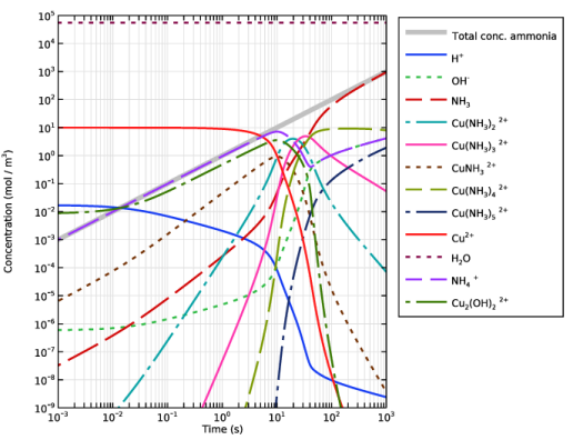
Locate the Plot Settings section.
|
|
4
|
Select the y-axis label checkbox. In the associated text field, type Concentration (mol / m<sup>3</sup>).
|
|
5
|
|
6
|
|
7
|
|
8
|
|
9
|
|
10
|
Select the x-axis log scale checkbox.
|
|
11
|
Select the y-axis log scale checkbox.
|
|
12
|
|
1
|
|
2
|
|
3
|
|
5
|
Click to expand the Coloring and Style section. Find the Line style subsection. From the Line list, choose Cycle.
|
|
6
|
|
7
|
|
1
|
|
2
|
|
4
|
|
5
|
|
6
|
Drag and drop above Species concentrations.
|
|
7
|
|
8
|
Clear the Expression checkbox.
|
|
9
|
|
1
|
|
2
|
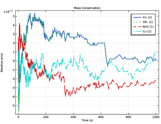
In the Settings window for Global Evaluation, type Relative Conservation Errors in the Label text field.
|
|
3
|
|
5
|
|
1
|
Go to the Evaluation Group 1 window.
|
|
2
|
Click the Clear Table button in the window toolbar.
|
|
1
|
|
2
|
|
3
|
|
1
|
|
2
|
|
3
|
|
4
|
Locate the Plot Settings section.
|
|
5
|
|
1
|
|
2
|
|
3
|
|
4
|
|
5
|
|
1
|
|
2
|
|
3
|
|
4
|
|
5
|
|
6
|
|
7
|
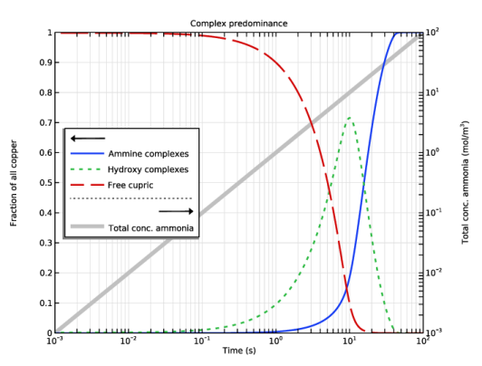
Select the Secondary y-axis log scale checkbox.
|
|
8
|
Select the Manual axis limits checkbox.
|
|
9
|
|
10
|
|
11
|
|
12
|
|
13
|
|
14
|
|
1
|
|
2
|
|
3
|
|
5
|
|
6
|
|
7
|
|
8
|
|
9
|
Clear the Expression checkbox.
|
|
1
|
|
2
|
|
4
|
Locate the Coloring and Style section. Find the Line style subsection. From the Line list, choose Cycle.
|
|
5
|
|
6
|
|
7
|
Clear the Expression checkbox.
|
|
8
|