PDF

Oscillations in Metabolic Reaction Networks
Introduction
Oscillating chemical reactions were long thought to simply not exist in homogeneous solution, and even the poster child, the Belousov–Zhabotinsky reaction, met such an initial skepticism, that even though it was discovered in 1951, it took almost 20 years for it to gain widespread fame. Since this seminal discovery, many more oscillating reaction networks have been discovered, and this model studies the oscillatory behavior of a key part of glycolysis, the ubiquitous metabolic pathway common to a large part of the living organisms on earth.
Model Definition
It has been found that yeast cells, if first starved, and then subjected to small amounts of cyanide, and replenished with glucose, starts to consume the glucose at an oscillating rate. The fact that the variation in concentrations of metabolites can be measured macroscopically, means that the phase of the oscillations in individual yeast cells synchronize among billions of cells. This communication between cells occurs via molecular transport across cell membranes. The setup here models this intercellular transport via a fixed flux of glucose into the cell, acetaldehyde out of the cell, and an equilibrium of acetaldehyde across the cell membrane.
The minimal chemical reaction network presented in Ref. 1, which is formed by a subset of the glycolysis, is set up using 11 species in a Reaction Engineering interface. A 0D component, with a Reaction Engineering interface, is used to describe the reactions in the cytoplasm of the yeast cell. The individual reactions, and how they map to the reaction network is presented in Figure 1. A possible extension of this model could be to set up explicit cell membranes and solve the problem using a component in a higher dimension, resolving diffusion spatially.
Figure 1: The relation between the reaction network and the features added to the Reaction Engineering interface.
Abbreviations for the metabolites are introduced for ease of input and brevity. The mappings of short names to their respective compound(s) are listed in Table 1.
Note how S3 represents a pool of metabolites, this is due to the model using lumped reactions to keep the number of variables low, while still reproducing the key features of the system.
Kinetics
Most reactions in the network are assigned mass action law expressions, the most prominent exception is that of the first reaction, where enzyme inhibition leads to a slightly more complicated expression, where a nonlinear factor enters the rate expression:
(1)
The final rate expressions are shown in Table 2. The influx of glucose into the cell is accounted for using an additional source.
The stoichiometric coefficients associated with each rate expression are given in Figure 1.
Parameters
The parameter values associated with the kinetic model are presented in Table 3.
The model is solved for a duration of 5 minutes using the time-dependent solver.
Results and Discussion
The result of the time integration is shown in Figure 2. Note how large the oscillations are in relative terms for glucose (S1).
Figure 2: Time evolution of concentrations.
Figure 3 highlights the covariation between ATP and NADH.
Figure 3: Time evolution of ATP and NAHD.
Note how the phases between ATP and NADH are offset by almost 180°. In this case, we can confirm the validity of our results by confirming that we reproduce the results of the referenced journal article. But more often than not, such a reference is not available, and hence it is never a bad idea to check how well the numerical solution respects invariants. Figure 4 shows how accurately mass conservation is fulfilled for ATP/ADP and NADH/NAD+. Note that the error is minuscule and on the order of machine precision.
Figure 4: Mass conservation of ATP/ADP and NADH/NAD+ over time.
Reference
1. J. Wolf and others, “Transduction of Intracellular and Intercellular Dynamics in Yeast Glycolytic Oscillations,” Biophysical Journal, vol. 78, pp. 1145–1153, 2000.
Application Library path: Chemical_Reaction_Engineering_Module/Ideal_Tank_Reactors/glycolytic_oscillations
Modeling Instructions
From the File menu, choose New.
New
In the New window, click  Model Wizard.
Model Wizard
1
In the Model Wizard window, click  0D.
2
In the Select Physics tree, select Chemical Species Transport > Reaction Engineering (re).
3
4
Click  Study.
5
In the Select Study tree, select General Studies > Time Dependent.
6
Reaction Engineering (re)
1
In the Model Builder window, under Component 1 (comp1) click Reaction Engineering (re).
2
In the Settings window for Reaction Engineering, locate the Mixture Properties section.
3
From the Phase list, choose Liquid.
Global Definitions
Parameters 1
Read in a set of parameters to be used in the model (naming matches terminology in referenced paper).
1
In the Model Builder window, under Global Definitions click Parameters 1.
2
In the Settings window for Parameters, locate the Parameters section.
3
Click  Load from File.
4
Definitions
Variables 1
1
In the Model Builder window, under Component 1 (comp1) right-click Definitions and choose Variables.
2
In the Settings window for Variables, locate the Variables section.
3
Click  Load from File.
4
Reaction Engineering (re)
Reaction 1
1
In the Reaction Engineering toolbar, click  Reaction.
2
In the Settings window for Reaction, locate the Reaction Formula section.
3
In the Formula text field, type S1+2A3=>S2+2A2.
4
Locate the Reaction Rate section. From the list, choose User defined.
5
In the rj text field, type k1*re.c_S1*re.c_A3*f_A3.
6
Locate the Reaction Orders section. Find the Volumetric overall reaction order subsection. In the Forward text field, type 2.
Additional Source - J0
1
In the Reaction Engineering toolbar, click  Additional Source.
2
In the Settings window for Additional Source, type Additional Source - J0 in the Label text field.
3
Locate the Additional Rate Expression section. In the Volumetric species table, enter the following settings:
Reaction 2
1
In the Reaction Engineering toolbar, click  Reaction.
2
In the Settings window for Reaction, locate the Reaction Formula section.
3
In the Formula text field, type S2=>2S3.
4
Locate the Rate Constants section. In the kf text field, type k2.
Reaction 3
1
In the Reaction Engineering toolbar, click  Reaction.
2
In the Settings window for Reaction, locate the Reaction Formula section.
3
In the Formula text field, type A2+N1+S3<=>A3+N2+S4.
4
Locate the Rate Constants section. In the kf text field, type k3fwd.
5
In the kr text field, type k3rev.
Reaction 4
1
In the Reaction Engineering toolbar, click  Reaction.
2
In the Settings window for Reaction, locate the Reaction Formula section.
3
In the Formula text field, type S4+A2=>S5+A3.
4
Locate the Rate Constants section. In the kf text field, type k4.
Reaction 5
1
In the Reaction Engineering toolbar, click  Reaction.
2
In the Settings window for Reaction, locate the Reaction Formula section.
3
In the Formula text field, type S5=>S6.
4
Locate the Rate Constants section. In the kf text field, type k5.
Reaction 6
1
In the Reaction Engineering toolbar, click  Reaction.
2
In the Settings window for Reaction, locate the Reaction Formula section.
3
In the Formula text field, type S6+N2=>N1.
4
Locate the Rate Constants section. In the kf text field, type k6.
Reaction 7
1
In the Reaction Engineering toolbar, click  Reaction.
2
In the Settings window for Reaction, locate the Reaction Formula section.
3
In the Formula text field, type A3=>A2.
4
Locate the Rate Constants section. In the kf text field, type k7.
Reaction 8
1
In the Reaction Engineering toolbar, click  Reaction.
2
In the Settings window for Reaction, locate the Reaction Formula section.
3
In the Formula text field, type S3+N2=>N1.
4
Locate the Rate Constants section. In the kf text field, type k8.
Reaction 9
1
In the Reaction Engineering toolbar, click  Reaction.
2
In the Settings window for Reaction, locate the Reaction Formula section.
3
In the Formula text field, type S6ex=>0S6ex.
4
Locate the Rate Constants section. In the kf text field, type k9.
J: S6<=>0.1S6ex
1
In the Reaction Engineering toolbar, click  Reaction.
2
In the Settings window for Reaction, locate the Reaction Formula section.
3
In the Formula text field, type S6<=>0.1S6ex.
4
In the Label text field, type J: S6<=>0.1S6ex.
5
Locate the Reaction Rate section. In the rj text field, type kappa*(re.c_S6-re.c_S6ex).
6
Locate the Reaction Orders section. Find the Volumetric overall reaction order subsection. In the Forward text field, type 1.
Initial Values 1
1
In the Model Builder window, click Initial Values 1.
2
In the Settings window for Initial Values, locate the Volumetric Species Initial Values section.
3
Study 1
Step 1: Time Dependent
1
In the Model Builder window, under Study 1 click Step 1: Time Dependent.
2
In the Settings window for Time Dependent, locate the Study Settings section.
3
In the Output times text field, type range(0,0.01,5).
4
From the Time unit list, choose min.
5
In the Study toolbar, click  Compute.
6
Click  Compute.
Results
Concentration (re)
1
In the Settings window for 1D Plot Group, click to expand the Title section.
2
From the Title type list, choose None.
3
Locate the Legend section. From the Layout list, choose Outside graph axis area.
Global 1
1
In the Model Builder window, expand the Concentration (re) node, then click Global 1.
2
In the Settings window for Global, click to expand the Coloring and Style section.
3
Find the Line style subsection. From the Line list, choose Cycle.
This is Figure 2.
Concentration (re) ATP and NADH vs. Time
1
In the Model Builder window, right-click Concentration (re) and choose Duplicate.
2
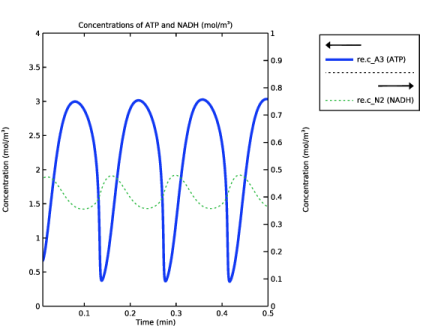
In the Settings window for 1D Plot Group, type Concentration (re) ATP and NADH vs. Time in the Label text field.
3
Locate the Title section. From the Title type list, choose Manual.
4
In the Title text area, type Concentrations of ATP and NADH (mol/m<sup>3</sup>).
5
Locate the Plot Settings section. Select the Two y-axes checkbox.
6
Locate the Axis section. Select the Manual axis limits checkbox.
7
In the x minimum text field, type 0.01.
8
In the x maximum text field, type 0.5.
9
In the y minimum text field, type 0.
10
In the y maximum text field, type 4.
11
In the Secondary y minimum text field, type 0.
12
Locate the Grid section. Clear the Show grid checkbox.
13
Locate the Legend section. From the Layout list, choose Outside graph axis area.
Global 1
1
In the Model Builder window, expand the Concentration (re) ATP and NADH vs. Time node, then click Global 1.
2
In the Settings window for Global, locate the y-Axis Data section.
3
Click  Clear Table.
4
Global 2
1
Right-click Results > Concentration (re) ATP and NADH vs. Time > Global 1 and choose Duplicate.
2
In the Settings window for Global, locate the y-Axis section.
3
Select the Plot on secondary y-axis checkbox.
4
Locate the y-Axis Data section. In the table, enter the following settings:
5
Click to expand the Legends section. From the Legends list, choose Manual.
6
Global 1
1
In the Model Builder window, click Global 1.
2
In the Settings window for Global, locate the Coloring and Style section.
3
From the Width list, choose 3.
4
Locate the Legends section. From the Legends list, choose Manual.
5
6
In the Concentration (re) ATP and NADH vs. Time toolbar, click  Plot.
This is Figure 3.
Mass Conservation A and N
1
In the Model Builder window, right-click Concentration (re) and choose Duplicate.
2
In the Settings window for 1D Plot Group, type Mass Conservation A and N in the Label text field.
3
Locate the Title section. From the Title type list, choose None.
4
Locate the Legend section. From the Layout list, choose Outside graph axis area.
Global 1
1
In the Model Builder window, expand the Mass Conservation A and N node, then click Global 1.
2
In the Settings window for Global, locate the y-Axis Data section.
3
Click  Clear Table.
4
5
In the Mass Conservation A and N toolbar, click  Plot.
This is Figure 4.