|
|
|
|
1
|
|
2
|
In the Select Physics tree, select Chemical Species Transport > Vapor–Liquid Equilibrium > Laminar Vapor Flow.
|
|
3
|
Click Add.
|
|
4
|
|
5
|
In the Mass fractions (1) table, enter the following settings:
|
|
6
|
|
7
|
Click Add.
|
|
8
|
Click
|
|
9
|
|
10
|
Click
|
|
1
|
|
2
|
|
3
|
Click
|
|
4
|
Browse to the model’s Application Libraries folder and double-click the file ethanol_water_evaporation_parameters.txt.
|
|
1
|
Go to the Select System window.
|
|
2
|
|
3
|
Click the Next button in the window toolbar.
|
|
1
|
Go to the Select Species window.
|
|
2
|
|
3
|
Click
|
|
4
|
|
5
|
Click
|
|
6
|
|
7
|
Click
|
|
8
|
Click the Next button in the window toolbar.
|
|
1
|
Go to the Select Thermodynamic Model window.
|
|
2
|
From the list, choose UNIQUAC.
|
|
3
|
Click the Finish button in the window toolbar.
|
|
1
|
Right-click Global Definitions > Thermodynamics > Vapor–Liquid System 1 (pp1) and choose Generate Chemistry.
|
|
1
|
Go to the Select Species window.
|
|
2
|
Click
|
|
3
|
Click the Next button in the window toolbar.
|
|
1
|
Go to the Chemistry Settings window.
|
|
2
|
|
3
|
Click the Finish button in the window toolbar.
|
|
1
|
|
2
|
|
3
|
Find the Bulk species subsection. From the Species solved for list, choose Transport of Concentrated Species in Vapor.
|
|
1
|
|
2
|
Browse to the model’s Application Libraries folder and double-click the file ethanol_water_evaporation_geom_sequence.mph.
|
|
3
|
|
1
|
In the Model Builder window, expand the Component 1 (comp1) > Multiphysics node, then click Reacting Flow 1 (nirf1).
|
|
2
|
|
3
|
|
4
|
|
1
|
|
2
|
|
3
|
|
1
|
|
2
|
In the Settings window for Variables, type Vapor-liquid interface variables in the Label text field.
|
|
3
|
|
4
|
Browse to the model’s Application Libraries folder and double-click the file ethanol_water_evaporation_interface_variables.txt.
|
|
1
|
In the Model Builder window, under Global Definitions > Thermodynamics right-click Vapor–Liquid System 1 (pp1) and choose Generate Material.
|
|
1
|
Go to the Select Phase window.
|
|
2
|
From the list, choose Liquid.
|
|
3
|
Click the Next button in the window toolbar.
|
|
1
|
Go to the Select Species window.
|
|
2
|
Click
|
|
3
|
|
4
|
Click
|
|
5
|
|
6
|
Click the Next button in the window toolbar.
|
|
1
|
Go to the Select Properties window.
|
|
2
|
Click the Next button in the window toolbar.
|
|
1
|
Go to the Define Material window.
|
|
2
|
Click the Finish button in the window toolbar.
|
|
1
|
In the Model Builder window, expand the Component 1 (comp1) > Materials node, then click Liquid: ethanol-water 1 (pp1mat1).
|
|
2
|
|
3
|
|
4
|
Locate the Material Contents section. Find the Local properties subsection. In the table, enter the following settings:
|
|
1
|
|
2
|
Go to the Add Material window.
|
|
3
|
|
4
|
Click Search.
|
|
5
|
|
6
|
Click the Add to Component button in the window toolbar.
|
|
7
|
|
8
|
Click Search.
|
|
9
|
|
10
|
Click the Add to Component button in the window toolbar.
|
|
11
|
|
1
|
|
2
|
|
1
|
|
2
|
|
3
|
|
1
|
In the Model Builder window, under Component 1 (comp1) click Transport of Concentrated Species in Vapor (tcs).
|
|
2
|
In the Settings window for Transport of Concentrated Species in Vapor, locate the Domain Selection section.
|
|
3
|
|
4
|
|
1
|
In the Model Builder window, expand the Transport of Concentrated Species in Vapor (tcs) node, then click Fluid 1.
|
|
2
|
|
3
|
|
4
|
Locate the Diffusion section. In the table, enter the following settings:
|
|
1
|
|
2
|
|
3
|
|
4
|
|
2
|
|
3
|
|
4
|
|
5
|
|
6
|
Select the wW, H2O (water) checkbox.
|
|
7
|
Locate the Liquid Phase section. From the Liquid phase concentration type list, choose Volume fraction.
|
|
9
|
|
10
|
In the Show More Options dialog, in the tree, select the checkbox for the node Physics > Advanced Physics Options.
|
|
11
|
Click OK.
|
|
12
|
|
13
|
|
1
|
|
2
|
|
3
|
|
4
|
Locate the Physical Model section. From the Compressibility list, choose Compressible flow (Ma<0.3).
|
|
5
|
Select the Include gravity checkbox.
|
|
6
|
|
1
|
|
2
|
|
4
|
|
1
|
In the Model Builder window, expand the Component 1 (comp1) > Heat Transfer in Fluids (ht) node, then click Initial Values 1.
|
|
2
|
|
3
|
|
1
|
|
1
|
|
2
|
|
3
|
|
4
|
|
1
|
|
3
|
|
4
|
|
1
|
|
2
|
|
3
|
From the list, choose User-controlled mesh.
|
|
1
|
|
2
|
|
3
|
|
4
|
|
6
|
|
7
|
|
8
|
Click the Custom button.
|
|
9
|
Locate the Element Size Parameters section.
|
|
10
|
|
1
|
|
2
|
|
3
|
|
4
|
|
6
|
|
7
|
|
8
|
Click the Custom button.
|
|
9
|
Locate the Element Size Parameters section.
|
|
10
|
|
1
|
|
2
|
|
3
|
|
5
|
|
6
|
|
7
|
Click the Custom button.
|
|
8
|
Locate the Element Size Parameters section.
|
|
9
|
|
1
|
|
1
|
In the Model Builder window, expand the Boundary Layers 1 node, then click Boundary Layer Properties 1.
|
|
3
|
|
4
|
|
5
|
|
6
|
Click
|
|
2
|
|
3
|
|
4
|
|
1
|
|
2
|
|
3
|
|
4
|
|
6
|
|
7
|
|
1
|
|
2
|
Drag and drop below Size.
|
|
3
|
|
4
|
|
1
|
|
2
|
|
3
|
|
4
|
|
5
|
Click the Custom button.
|
|
6
|
Locate the Element Size Parameters section.
|
|
7
|
|
1
|
|
2
|
|
3
|
|
5
|
|
6
|
|
7
|
Click the Custom button.
|
|
8
|
Locate the Element Size Parameters section.
|
|
9
|
|
10
|
Click
|
|
1
|
|
2
|
|
3
|
|
5
|
|
6
|
Locate the Element Size Parameters section.
|
|
7
|
|
8
|
Click
|
|
9
|
Click
|
|
1
|
|
2
|
|
3
|
|
4
|
Click
|
|
1
|
|
2
|
|
3
|
In the Output times text field, type range(0,0.1,1) range(1.25,0.25,4) range(5,1,20) range(25,5,120) range(130,10,240) range(270,30,900).
|
|
1
|
In the Model Builder window, expand the Study 1 > Solver Configurations > Solution 1 (sol1) > Dependent Variables 1 node, then click Temperature (comp1.T).
|
|
2
|
|
3
|
|
4
|
|
5
|
In the Model Builder window, under Study 1 > Solver Configurations > Solution 1 (sol1) > Dependent Variables 1 click Velocity Field (comp1.u).
|
|
6
|
|
7
|
|
8
|
|
9
|
In the Model Builder window, under Study 1 > Solver Configurations > Solution 1 (sol1) > Dependent Variables 1 click Mass Fraction (comp1.wEth).
|
|
10
|
|
11
|
|
12
|
In the Model Builder window, under Study 1 > Solver Configurations > Solution 1 (sol1) > Dependent Variables 1 click Mass Fraction (comp1.wW).
|
|
13
|
|
14
|
|
1
|
In the Model Builder window, under Study 1 > Solver Configurations > Solution 1 (sol1) click Time-Dependent Solver 1.
|
|
2
|
|
3
|
Select the Initial step checkbox.
|
|
4
|
In the Study toolbar, click
|
|
1
|
|
2
|
|
3
|
|
1
|
|
2
|
|
3
|
Click
|
|
4
|
|
5
|
|
6
|
Click OK.
|
|
7
|
|
9
|
Click
|
|
1
|
|
2
|
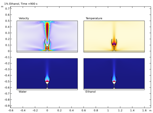
In the Settings window for 2D Plot Group, type Array: Velocity, Temperature, and Mass Fractions in the Label text field.
|
|
3
|
|
4
|
Click to expand the Title section. Locate the Color Legend section. Select the Show maximum and minimum values checkbox.
|
|
5
|
Select the Show units checkbox.
|
|
6
|
|
7
|
|
8
|
|
9
|
|
10
|
|
11
|
|
1
|
|
2
|
|
3
|
|
1
|
|
2
|
|
3
|
|
4
|
|
5
|
|
6
|
|
1
|
|
2
|
|
3
|
|
4
|
|
5
|
|
6
|
|
1
|
|
2
|
|
3
|
|
4
|
|
5
|
|
6
|
|
1
|
|
2
|
|
3
|
|
1
|
In the Model Builder window, right-click Array: Velocity, Temperature, and Mass Fractions and choose Arrow Surface.
|
|
2
|
|
3
|
|
4
|
|
5
|
|
6
|
|
7
|
|
8
|
|
9
|
|
10
|
|
1
|
In the Model Builder window, right-click Array: Velocity, Temperature, and Mass Fractions and choose Annotation.
|
|
2
|
|
3
|
|
4
|
|
5
|
|
6
|
|
7
|
|
8
|
|
1
|
|
2
|
|
3
|
|
4
|
|
1
|
|
2
|
|
3
|
|
4
|
|
5
|
|
1
|
|
2
|
|
3
|
|
4
|
|
5
|
|
1
|
|
2
|
|
3
|
Select the Plot checkbox.
|
|
5
|
|
1
|
|
2
|
|
3
|
Select the Plot checkbox.
|
|
1
|
|
2
|
|
3
|
|
1
|
|
2
|
|
3
|
|
4
|
|
5
|
|
6
|
|
7
|
|
8
|
|
1
|
|
2
|
|
3
|
Locate the Expression section. In the Expression text field, type withsol('sol2',spf.U,setval(abv,0.01,t,t)).
|
|
4
|
|
1
|
|
2
|
|
3
|
Locate the Expression section. In the Expression text field, type withsol('sol2',spf.U,setval(abv,0.15,t,t)).
|
|
4
|
|
5
|
|
6
|
|
7
|
|
1
|
|
2
|
|
3
|
Locate the Expression section. In the Expression text field, type withsol('sol2',spf.U,setval(abv,0.4,t,t)).
|
|
4
|
|
5
|
|
6
|
|
1
|
|
2
|
|
3
|
Locate the Expression section. In the Expression text field, type withsol('sol2',spf.U,setval(abv,0.99,t,t)).
|
|
4
|
|
5
|
|
1
|
|
2
|
|
3
|
Locate the Expression section. In the x-component text field, type withsol('sol2',u,setval(abv,0.01,t,t)).
|
|
4
|
|
5
|
Locate the Arrow Positioning section. Find the x grid points subsection. In the Points text field, type 12.
|
|
6
|
|
7
|
|
8
|
|
9
|
|
10
|
|
11
|
|
1
|
|
2
|
|
3
|
Locate the Expression section. In the x-component text field, type withsol('sol2',u,setval(abv,0.15,t,t)).
|
|
4
|
|
5
|
|
1
|
|
2
|
|
3
|
Locate the Expression section. In the x-component text field, type withsol('sol2',u,setval(abv,0.4,t,t)).
|
|
4
|
|
5
|
|
6
|
|
1
|
|
2
|
|
3
|
Locate the Expression section. In the x-component text field, type withsol('sol2',u,setval(abv,0.99,t,t)).
|
|
4
|
|
5
|
|
6
|
|
7
|
|
1
|
|
2
|
|
3
|
|
4
|
|
5
|
|
1
|
|
2
|
|
3
|
|
4
|
|
5
|
|
6
|
|
7
|
|
8
|
|
9
|
|
1
|
|
2
|
|
3
|
|
4
|
|
5
|
|
1
|
|
2
|
|
3
|
|
4
|
|
5
|
|
6
|
|
1
|
|
2
|
|
3
|
|
4
|
|
5
|
|
1
|
|
2
|
|
3
|
|
1
|
|
2
|
|
3
|
|
4
|
|
5
|
Locate the Expressions section. In the table, enter the following settings:
|
|
6
|
|
1
|
|
2
|
|
3
|
|
4
|
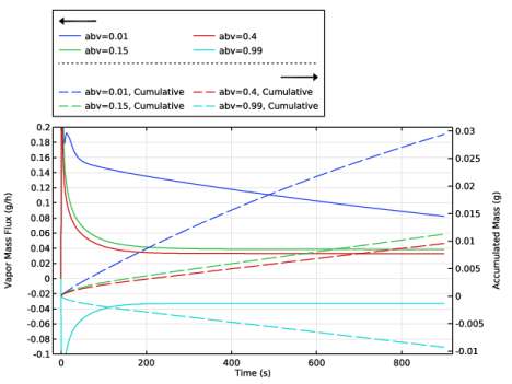
Select the Cumulative checkbox.
|
|
5
|
|
1
|
|
2
|
|
3
|
|
4
|
|
5
|
|
6
|
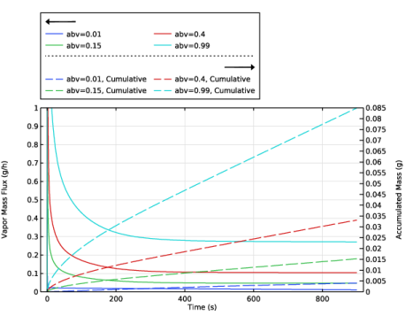
In the Columns list, choose abv=0.01, -tcs.ntflux_wW (g/h), abv=0.15, -tcs.ntflux_wW (g/h), abv=0.4, -tcs.ntflux_wW (g/h), and abv=0.99, -tcs.ntflux_wW (g/h).
|
|
7
|
|
1
|
|
2
|
|
3
|
Locate the Plot Settings section.
|
|
4
|
|
5
|
Select the Two y-axes checkbox.
|
|
6
|
Select the Secondary y-axis label checkbox. In the associated text field, type Accumulated Mass (g).
|
|
7
|
|
8
|
|
9
|
|
10
|
|
1
|
|
2
|
|
3
|
In the Columns list, choose abv=0.01, Cumulative integral: -tcs.ntflux_wW (g), abv=0.15, Cumulative integral: -tcs.ntflux_wW (g), abv=0.4, Cumulative integral: -tcs.ntflux_wW (g), and abv=0.99, Cumulative integral: -tcs.ntflux_wW (g).
|
|
4
|
Locate the Coloring and Style section. Find the Line style subsection. From the Line list, choose Dashed.
|
|
5
|
|
6
|
|
1
|
|
2
|
|
3
|
Select the Manual axis limits checkbox.
|
|
4
|
|
5
|
|
6
|
|
1
|
|
2
|
|
3
|
|
1
|
|
2
|
In the Settings window for Line Integration, click Replace Expression in the upper-right corner of the Expressions section. From the menu, choose Component 1 (comp1) > Transport of Concentrated Species in Vapor > Species wEth > Fluxes > tcs.ntflux_wEth - Normal total flux - kg/(m²·s).
|
|
3
|
Locate the Expressions section. In the table, enter the following settings:
|
|
1
|
|
2
|
In the Settings window for Line Integration, click Replace Expression in the upper-right corner of the Expressions section. From the menu, choose tcs.ntflux_wEth - Normal total flux - kg/(m²·s).
|
|
3
|
Locate the Expressions section. In the table, enter the following settings:
|
|
4
|
|
1
|
|
2
|
|
1
|
|
2
|
|
3
|
|
1
|
|
2
|
|
3
|
|
4
|
|
1
|
|
2
|
|
3
|
Select the Manual axis limits checkbox.
|
|
4
|
|
5
|
|
6
|
|
7
|
|
1
|
|
2
|
In the Settings window for Evaluation Group, type Evaluation: Kinetic Energy in the Label text field.
|
|
3
|
|
1
|
|
2
|
|
3
|
|
4
|
|
5
|
Locate the Expressions section. In the table, enter the following settings:
|
|
6
|
|
1
|
|
2
|
|
3
|
|
4
|
Locate the Plot Settings section.
|
|
5
|
|
6
|
|
1
|
|
2
|
|
3
|
|
4
|
|
5
|
|
6
|
|
7
|
|
8
|
Click
|
|
1
|
|
2
|
|
3
|
|
4
|
|
1
|
|
3
|
|
4
|
|
5
|
|
6
|
|
7
|
|
8
|
|
1
|
|
2
|
In the Settings window for 1D Plot Group, type Surface Concentration Ethanol in the Label text field.
|
|
1
|
In the Model Builder window, expand the Surface Concentration Ethanol node, then click Point Graph 1.
|
|
2
|
|
3
|
Click to select the
|
|
5
|
Click Replace Expression in the upper-right corner of the y-Axis Data section. From the menu, choose Component 1 (comp1) > Transport of Concentrated Species in Vapor > Species wEth > tcs.c_wEth - Molar concentration - mol/m³.
|
|
6
|
|
1
|
|
2
|
|
3
|
|
1
|
|
2
|
|
3
|
|
4
|
|
1
|
|
2
|
|
3
|
|
4
|
|
1
|
|
2
|
|
3
|
|
4
|
|
5
|
|
6
|
|
7
|
|
1
|
|
2
|
|
3
|
|
4
|
|
5
|
|
1
|
|
2
|
|
3
|
|
4
|
|
5
|
Click Define custom colors.
|
|
7
|
Click Add to custom colors.
|
|
8
|
|
9
|
|
10
|
Click Define custom colors.
|
|
12
|
Click Add to custom colors.
|
|
13
|
|
14
|
|
15
|
Click Define custom colors.
|
|
17
|
Click Add to custom colors.
|
|
18
|
|
19
|
Select the Normal mapping checkbox.
|
|
20
|
|
21
|
|
22
|
Select the Additional color checkbox.
|
|
23
|
|
24
|
|
25
|
|
26
|
Click Define custom colors.
|
|
28
|
Click Add to custom colors.
|
|
29
|
|
30
|
|
31
|
|
32
|
|
33
|
|
34
|
|
35
|
|
36
|
|
37
|
|
1
|
In the Model Builder window, expand the Study 1/Parametric Solutions 1 (4) (sol2) node, then click Selection.
|
|
1
|
|
2
|
|
3
|
|
1
|
|
2
|
|
3
|
|
4
|
|
5
|
|
1
|
|
2
|
|
3
|
|
4
|
|
1
|
|
2
|
|
3
|
|
1
|
|
2
|
|
3
|
|
4
|
|
5
|
|
1
|
|
2
|
|
3
|
|
4
|
|
1
|
|
2
|
|
3
|
|
4
|
|
5
|
|
6
|
|
7
|
|
8
|
|
9
|
|
10
|
|
11
|
|
1
|
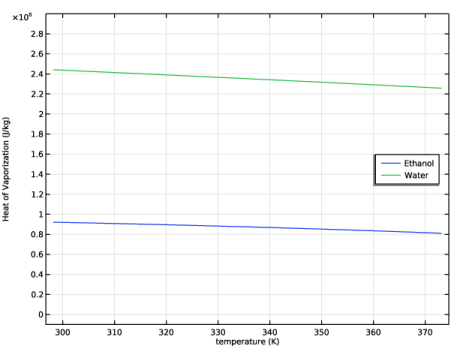
In the Model Builder window, expand the Global Definitions > Thermodynamics > Vapor–Liquid System 1 (pp1) > ethanol node, then click Heat of vaporization 1 (chempp1dHvap_ethanol, chempp1dHvap_ethanol_Dtemperature).
|
|
2
|
|
1
|
In the Model Builder window, expand the Global Definitions > Thermodynamics > Vapor–Liquid System 1 (pp1) > water node, then click Heat of vaporization 2 (chempp1dHvap_water, chempp1dHvap_water_Dtemperature).
|
|
2
|
|
1
|
|
2
|
|
3
|
|
4
|
|
1
|
|
2
|
|
3
|
|
4
|
|
1
|
|
2
|
|
3
|
|
4
|
Locate the Plot Settings section.
|
|
5
|
|
6
|
|
7
|
|
8
|
|
9
|
|
10
|
|
1
|
|
2
|
|
3
|
Click
|
|
1
|
|
2
|
|
3
|
|
4
|
|
1
|
|
2
|
|
3
|
|
4
|
|
1
|
|
2
|
|
3
|
|
4
|
|
1
|
In the Model Builder window, under Component 1 (comp1) > Geometry 1, Ctrl-click to select Point 1 (pt1) and Point 2 (pt2).
|
|
2
|
Right-click and choose Group.
|
|
1
|
|
2
|
|
3
|
|
4
|
|
1
|
|
2
|
|
3
|
|
4
|
|
1
|
|
2
|
|
3
|
|
4
|
|
1
|
|
2
|
|
3
|
|
4
|
|
1
|
|
2
|
|
3
|
|
4
|
|
1
|
|
2
|
|
3
|
|
4
|
|
1
|
|
2
|
|
3
|
|
4
|
|
1
|
|
2
|
|
3
|
Click
|
|
1
|
|
2
|
|
3
|
|
4
|
Locate the Coordinates section. In the table, enter the following settings:
|
|
1
|
|
2
|
|
3
|
|
4
|
|
5
|
|
6
|
|
7
|
|
8
|
|
1
|
|
2
|
|
3
|
|
4
|
|
5
|
|
6
|
|
7
|
|
8
|
|
1
|
In the Model Builder window, under Component 1 (comp1) > Geometry 1 right-click Circular Arc 1 (ca1) and choose Duplicate.
|
|
2
|
|
3
|
|
4
|
|
1
|
|
2
|
|
3
|
|
1
|
|
2
|
Select the object uni1 only.
|
|
3
|
|
1
|
|
2
|
On the object csol1, select Points 16 and 17 only.
|
|
3
|
|
4
|
|
1
|
|
2
|
|
1
|
|
2
|
Select the object pol2 only.
|
|
3
|
|
4
|
|
5
|
Select the object fil1 only.
|
|
6
|
Select the Keep objects to subtract checkbox.
|
|
1
|
|
2
|
|
1
|
In the Model Builder window, under Component 1 (comp1) > Geometry 1 right-click Difference 1 (dif1) and choose Duplicate.
|
|
2
|
|
3
|
|
4
|
Select the object pol3 only.
|
|
1
|
|
2
|
|
3
|
|
4
|
|
5
|
|
1
|
|
2
|
|
3
|
|
4
|
|
5
|
|
6
|
|
7
|
|
8
|
|
1
|
|
2
|
|
3
|
|
4
|
|
5
|
|
6
|
|
7
|
|
8
|
|
1
|
|
2
|
|
3
|
|
4
|
On the object pt3, select Point 1 only.
|
|
5
|
On the object pt4, select Point 1 only.
|
|
6
|
Click
|
|
1
|
|
2
|
|
3
|
|
4
|
On the object fin, select Point 25 only.
|
|
5
|
Locate the Vertex to Remove section. Click to select the
|
|
6
|
On the object fin, select Point 26 only.
|
|
7
|
|
1
|
|
2
|
On the object mrv1, select Boundaries 10, 24, and 26 only.
|
|
1
|
|
2
|
|
3
|
On the object mce1, select Domain 3 only.
|
|
1
|
|
2
|
|
3
|
On the object mce1, select Domain 2 only.
|
|
1
|
|
2
|
|
3
|
On the object mce1, select Domain 4 only.
|
|
1
|
|
2
|
|
3
|
On the object mce1, select Domain 1 only.
|
|
1
|
|
2
|
|
3
|
|
4
|
On the object mce1, select Boundary 8 only.
|
|
5
|