
|
|
|

|
1
|
|
2
|
|
3
|
Click Add.
|
|
4
|
|
5
|
Click Add.
|
|
6
|
|
7
|
Click Add.
|
|
8
|
Click
|
|
9
|
|
10
|
Click
|
|
1
|
|
2
|
|
3
|
Click
|
|
4
|
Browse to the model’s Application Libraries folder and double-click the file electroosmotic_flow_parameters.txt.
|
|
1
|
|
2
|
|
3
|
Click
|
|
4
|
Browse to the model’s Application Libraries folder and double-click the file electroosmotic_flow_variables.txt.
|
|
1
|
|
2
|
|
3
|
|
4
|
|
5
|
Browse to the model’s Application Libraries folder and double-click the file electroosmotic_flow.mph.
|
|
1
|
|
2
|
|
3
|
|
4
|
On the object dif1, select Boundaries 4, 5, 11, and 12 only.
|
|
1
|
|
2
|
|
3
|
|
4
|
On the object dif1, select Boundaries 7, 8, 13, and 14 only.
|
|
1
|
|
2
|
|
3
|
|
4
|
On the object dif1, select Boundary 1 only.
|
|
1
|
|
2
|
|
3
|
|
4
|
On the object dif1, select Boundary 10 only.
|
|
1
|
|
2
|
|
3
|
|
4
|
Locate the Constitutive Relation Jc-E section. From the σ list, choose User defined. In the associated text field, type kappa0.
|
|
5
|
|
1
|
|
2
|
|
3
|
|
1
|
|
2
|
|
3
|
|
4
|
|
1
|
|
2
|
|
3
|
|
4
|
|
5
|
|
6
|
Click OK.
|
|
7
|
|
8
|
In the Source term quantity table, enter the following settings:
|
|
9
|
|
10
|
In the Dependent variables (Pa) table, enter the following settings:
|
|
1
|
In the Model Builder window, under Component 1 (comp1) > Electroosmotic Pressure (g) click General Form PDE 1.
|
|
2
|
|
3
|
Specify the Γ vector as
|
|
4
|
|
5
|
|
1
|
|
2
|
|
3
|
|
1
|
|
2
|
In the Settings window for Dirichlet Boundary Condition, type Outlet - p=p1 in the Label text field.
|
|
3
|
|
4
|
|
1
|
|
2
|
|
3
|
Select the Migration in electric field checkbox.
|
|
1
|
In the Model Builder window, under Component 1 (comp1) > Transport of Diluted Species (tds) click Species Charges.
|
|
2
|
|
3
|
|
1
|
|
2
|
|
3
|
|
4
|
|
5
|
|
6
|
|
1
|
|
2
|
|
3
|
|
1
|
|
3
|
|
4
|
Select the Species c checkbox.
|
|
5
|
|
1
|
|
2
|
|
3
|
|
1
|
|
2
|
|
3
|
In the Solve for column of the table, under Component 1 (comp1), clear the checkbox for Transport of Diluted Species (tds).
|
|
1
|
|
2
|
|
3
|
|
4
|
|
5
|
|
6
|
Locate the Physics and Variables Selection section. In the Solve for column of the table, under Component 1 (comp1), clear the checkboxes for Electric Currents (ec) and Electroosmotic Pressure (g).
|
|
7
|
|
1
|
|
2
|
|
1
|
|
2
|
|
3
|
|
4
|
|
5
|
|
6
|
|
7
|
|
8
|
|
9
|
|
10
|
|
11
|
|
12
|
|
13
|
|
14
|
|
15
|
|
16
|
|
1
|
|
2
|
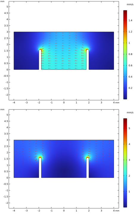
In the Settings window for 2D Plot Group, type Velocity Electroosmotic Term in the Label text field.
|
|
3
|
|
4
|
|
1
|
|
2
|
|
3
|
Click Replace Expression in the upper-right corner of the Expression section. From the menu, choose Component 1 (comp1) > Definitions > Variables > U_eo - Flow-velocity electroosmosis term, magnitude - m/s.
|
|
4
|
|
1
|
|
2
|
|
3
|
|
4
|
|
5
|
|
6
|
|
7
|
|
1
|
|
2
|
|
3
|
|
4
|
|
1
|
|
2
|
|
3
|
Click Replace Expression in the upper-right corner of the Expression section. From the menu, choose Component 1 (comp1) > Definitions > Variables > U_p - Velocity pressure term, magnitude - m/s.
|
|
4
|
|
1
|
|
2
|
|
3
|
|
4
|
|
5
|
|
6
|
|
7
|
|
1
|
|
2
|
|
3
|
|
4
|
|
1
|
|
2
|
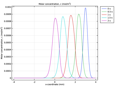
In the Settings window for 1D Plot Group, type Concentration Along x-axis @ y=2.5mm in the Label text field.
|
|
3
|
|
4
|
|
5
|
|
6
|
|
1
|
|
2
|
In the Settings window for Line Graph, click Replace Expression in the upper-right corner of the y-Axis Data section. From the menu, choose Component 1 (comp1) > Transport of Diluted Species > Species c > c - Molar concentration, c - mol/m³.
|
|
3
|
Click Replace Expression in the upper-right corner of the x-Axis Data section. From the menu, choose Component 1 (comp1) > Geometry > Coordinate > x - x-coordinate.
|
|
4
|
|
5
|
|
6
|
|
1
|
|
2
|