
|
|
|
|
1
|
|
2
|
|
3
|
Click Add.
|
|
4
|
Click
|
|
1
|
|
1
|
|
1
|
Go to the Select System window.
|
|
2
|
|
3
|
Click the Next button in the window toolbar.
|
|
1
|
Go to the Select Species window.
|
|
2
|
|
3
|
Click
|
|
4
|
|
5
|
Click
|
|
6
|
Click the Next button in the window toolbar.
|
|
1
|
Go to the Select Thermodynamic Model window.
|
|
2
|
From the list, choose NRTL.
|
|
3
|
Click the Finish button in the window toolbar.
|
|
1
|
|
2
|
|
3
|
Select the Thermodynamics checkbox.
|
|
4
|
Locate the Species Matching section. In the table, enter the following settings:
|
|
1
|
Go to the Select Species window.
|
|
2
|
Click
|
|
3
|
Click the Next button in the window toolbar.
|
|
1
|
Go to the Equilibrium Specifications window.
|
|
2
|
|
3
|
|
4
|
|
5
|
Click the Next button in the window toolbar.
|
|
1
|
Go to the Equilibrium Function Overview window.
|
|
2
|
Click the Finish button in the window toolbar.
|
|
1
|
|
2
|
|
3
|
Locate the Definition section. In the Expression text field, type Flash1_1_PhaseComposition_Vapor_ethanol(p,n,x1,x2).
|
|
4
|
|
5
|
Locate the Units section. In the table, enter the following settings:
|
|
6
|
|
1
|
|
2
|
|
3
|
Click
|
|
4
|
Browse to the model’s Application Libraries folder and double-click the file distillation_column_parameters.txt.
|
|
1
|
|
2
|
Go to the Add Study window.
|
|
3
|
Find the Physics interfaces in study subsection. In the table, clear the Solve checkbox for Reaction Engineering (re).
|
|
4
|
Find the Studies subsection. In the Select Study tree, select Preset Studies for Selected Physics Interfaces > Stationary.
|
|
5
|
Click the Add Study button in the window toolbar.
|
|
6
|
|
1
|
|
2
|
Select the Auxiliary sweep checkbox.
|
|
3
|
Click
|
|
5
|
Click
|
|
7
|
|
8
|
|
1
|
|
2
|
|
3
|
Click
|
|
5
|
|
6
|
|
7
|
|
1
|
|
2
|
|
3
|
|
4
|
Locate the Plot Settings section.
|
|
5
|
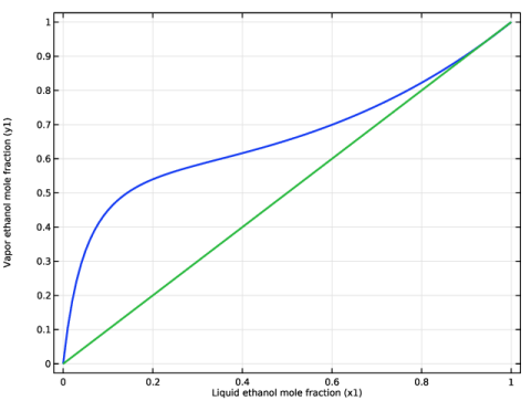
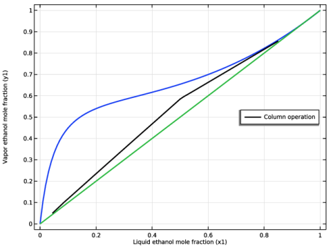
Select the x-axis label checkbox. In the associated text field, type Liquid ethanol mole fraction (x1).
|
|
6
|
Select the y-axis label checkbox. In the associated text field, type Vapor ethanol mole fraction (y1).
|
|
7
|
|
1
|
|
2
|
|
1
|
|
2
|
|
3
|
|
4
|
Locate the Physics Interfaces section. Find the Chemical species transport subsection. From the list, choose Transport of Concentrated Species: New.
|
|
5
|
|
1
|
|
2
|
|
3
|
|
5
|
Click
|
|
1
|
|
2
|
|
4
|
Click
|
|
5
|
|
1
|
In the Model Builder window, under Component 2 (comp2) click Transport of Concentrated Species (tcs).
|
|
2
|
|
3
|
|
4
|
|
1
|
Go to the Add Physics window.
|
|
2
|
|
3
|
Click to expand the Dependent Variables section. In the Mass fractions (1) table, enter the following settings:
|
|
4
|
Click the Add to Component 2 button in the window toolbar.
|
|
5
|
|
1
|
|
2
|
|
3
|
|
1
|
|
2
|
|
3
|
|
4
|
Click
|
|
5
|
Browse to the model’s Application Libraries folder and double-click the file distillation_column_variables.txt.
|
|
1
|
In the Model Builder window, under Component 2 (comp2) > Transport of Concentrated Species (tcs) click Fluid 1.
|
|
2
|
|
3
|
|
1
|
|
2
|
|
3
|
|
4
|
|
5
|
|
6
|
|
1
|
In the Model Builder window, under Component 2 (comp2) > Transport of Concentrated Species (tcs) click Fluid 1.
|
|
2
|
|
3
|
|
4
|
|
1
|
|
2
|
|
3
|
|
1
|
|
2
|
|
3
|
From the Chemistry list, choose User defined. From the RwE list, choose User defined. In the associated text field, type -tcs.M_wE*Kya*(ym1-ye1).
|
|
4
|
|
1
|
|
3
|
|
4
|
Select the Species wE checkbox.
|
|
5
|
|
1
|
|
1
|
In the Model Builder window, under Component 2 (comp2) > Transport of Concentrated Species 2 (tcs2) click Species Molar Masses 1.
|
|
2
|
|
3
|
|
4
|
|
1
|
|
2
|
|
3
|
Specify the u vector as
|
|
4
|
Locate the Diffusion section. In the table, enter the following settings:
|
|
1
|
|
2
|
|
3
|
|
1
|
In the Model Builder window, under Component 2 (comp2) > Transport of Concentrated Species 2 (tcs2) right-click Fluid 1 and choose Duplicate.
|
|
3
|
|
4
|
Specify the u vector as
|
|
1
|
|
3
|
|
4
|
Select the Species wEl checkbox.
|
|
5
|
|
1
|
|
3
|
|
4
|
Select the Species wEl checkbox.
|
|
5
|
|
1
|
|
1
|
|
2
|
|
3
|
|
4
|
|
5
|
|
6
|
Click in the Graphics window and then press Ctrl+A to select both domains.
|
|
1
|
|
2
|
|
3
|
|
4
|
Click in the Graphics window and then press Ctrl+A to select all boundaries.
|
|
5
|
|
6
|
|
7
|
Click
|
|
1
|
|
2
|
|
3
|
|
1
|
|
2
|
|
3
|
Click
|
|
5
|
|
1
|
|
2
|
|
3
|
|
4
|
|
5
|
|
1
|
|
2
|
|
3
|
|
4
|
|
5
|
|
6
|
|
7
|
|
1
|
|
2
|
|
3
|
|
4
|
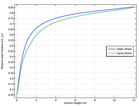
Locate the Legends section. In the table, enter the following settings:
|
|
5
|
|
1
|
|
2
|
|
3
|
|
4
|
Locate the Plot Settings section.
|
|
5
|
|
6
|
Select the y-axis label checkbox. In the associated text field, type Ethanol mole fraction (x1, y1).
|
|
7
|
|
8
|
|
1
|
|
2
|
|
3
|
|
4
|
|
5
|
|
1
|
|
2
|
|
3
|
|
4
|
|
5
|
|
6
|
|
7
|
|
8
|
|
9
|
|
10
|
|
12
|
|
1
|
|
2
|
|
3
|
Click
|
|
5
|
Locate the Data section. From the Dataset list, choose Equilibrium Curve Parameterization/Solution 1 (sol1).
|
|
6
|
|
7
|
|
8
|
|
9
|
|
10
|
|
1
|
|
2
|
|
3
|
|
4
|
Locate the Plot Settings section.
|
|
5
|
Select the x-axis label checkbox. In the associated text field, type Liquid ethanol mole fraction (x1).
|
|
6
|
Select the y-axis label checkbox. In the associated text field, type Vapor ethanol mole fraction (y1).
|
|
7
|
|
8
|