PDF

Dissociation in a Tubular Reactor
Introduction
Tubular reactors are often used in continuous large-scale production, for example in the petroleum industry. One key design and optimization parameter is the conversion, or the amount of reactant that reacts to form the desired product. In order to achieve high conversion, process engineers optimize the reactor design: its length, width, and heating system. An accurate reactor model is a very useful tool, both at the design stage and in tuning an existing reactor.
Figure 1: Dissociation reaction in a tubular reactor.
This example deals with a gas-phase dissociation process, species A reacts to form B (see Figure 1). The following physics interfaces are used:
Model Definition
Key Instructive Elements
This model illustrates several attractive features in the Chemical Reaction Engineering Module:
Handling Thermal and Transport Properties — Chemistry
The molecule N2O4 is a dimer which exists in a strongly temperature dependent equilibrium:
The kinetics of reaction is defined as
where kf denotes the forward reaction rate constant (SI unit: s1), c represents the concentration of species (SI unit: mol/m3) and Keq is the equilibrium constant (dimensionless).
The Chemistry interface coupled with Thermodynamics can provide all species and mixture thermal and transport properties. These properties can be used directly in other physics interfaces. Species and their properties can be selected from the COMSOL database.
The section Modeling Instructions, explains how to add a new species to this database, because nitrogen dioxide (NO2) and nitrogen tetroxide (N2O4) are not available.
Handling Expanding Flow — Compressible Flow formulation
Each mole of the reactant, A, reacts to form two moles of the product, B:
This leads to a volumetric expansion of the gas mixture as the reaction proceeds. The fluid’s change in density influences the gas velocity in the reactor, causing an acceleration as the reaction proceeds.
In order to model the flow, use a compressible formulation of the Navier–Stokes equations, defined according to the following equations:
Here ρ denotes the solution’s density (SI unit: kg/m3), u is the velocity vector (SI unit: m/s), p gives the pressure (SI unit: Pa), μ represents the solution’s viscosity (SI unit: kg/(m·s), or Pa·s), and I denotes the identity matrix.
The density is varying and depends on the pressure, temperature, and composition according to the ideal gas law. This is the default gas phase model, as defined in the Thermodynamics interface’s Gas System node under Thermodynamic Model. It is coupled to other interfaces in the model via the Chemistry interface’s Mixture Properties section.
The model applies the Laminar Flow interface, which solves the above equations, describing the momentum balances and the continuity (mass conservation) for fluids with variations in density.
Convection and Diffusion in Multicomponent Systems — Transport of Concentrated Species
As the dissociation reaction proceeds, the composition of the mixture changes from pure A at the inlet to a mixture of A and B.
The total mass flux is strongly influenced by the flux of each species. In addition, several molecular interactions occur; A interacts with B and other A molecules, B interacts with A and other B molecules. This implies that the simple Fick’s law formulation, with one constant diffusivity for each species is not applicable here. In a concentrated multicomponent mixture you must account for all possible interactions, and the flux is dependent on the fluid’s local composition. Simple Fick diffusivity accounts only for the interaction between solvent and solute. In the Transport of Concentrated Species with the Maxwell-Stefan or Mixture-Averaged diffusion equations, multicomponent diffusivities describe the interactions between all components in the system.
Since a change in a gas mixture composition affects the density, the species transport equation needs to be coupled with the flow equations (Laminar Flow, Navier–Stokes in this case).
Now consider a mathematical formulation of this discussion. The mass-balance equation for each species is
where wA and wB are the mass fractions of each component, nA and nB are the total fluxes of the species (including both convective and diffusive contributions), and RA and RB are given by the reaction kinetics from Chemistry interface. As mentioned earlier, it is possible to rewrite the mass-balances equations for each species by replacing one of the species’ mass balance with a total mass balance. A solution with two species follows following equation:
Because the system consists only of two species, the sum of wA and wB is always unity, and the sum of the reaction terms is zero. The above equation now becomes
which is the total mass-balance equation.
Geometry
The geometry of the tubular reactor is rotationally symmetric, and it is possible to reduce the model from 3D to a 2D axisymmetric problem. This means that you only have to model half of the tube cross section, as illustrated in Figure 2.
Figure 2: Model geometry.
Boundary conditions
Laminar Flow interface
The flow in the reactor is driven by Normal inflow velocity at inlet. The walls are represented by no slip boundary conditions u = 0.
Transport of Concentrated Species interface
At the inlet, the mass fraction of A is set close to unity (0.99). The outlet boundary condition is a convective flux condition. The convective flux condition implies that diffusive flux for the species is zero perpendicular to the boundary. This is a common assumption when modeling the outlet in tubular reactors.
No-flux conditions — referred to as insulation/symmetry in COMSOL Multiphysics —apply at all other boundaries. Across these boundaries a no (total) mass flux condition is prescribed for all species.
Mesh
In this example, a mapped (structured) mesh is a good choice due to the reactor’s regular shape. The use of a structured mesh is especially suitable when the requirements for the mesh density is uneven. In this example a denser mesh is required in the inlet region and the reactor wall. This is achieved by specifying the edge element distribution, as you see in Modeling Instructions.
Study 1 — Results and Discussion for Isothermal Conditions
Under isothermal conditions, the Laminar Flow and Transport of Concentrated Species interfaces, coupled using a Reacting Flow multiphysics node, are applied to solve the compressible Navier–Stokes equations together with mass transport equations including Maxwell-Stefan diffusion. The Chemistry interface defines the reactions kinetics as well as the transport properties of the fluid mixture. The binary diffusivity and the viscosity are defined dependent on the composition. The Reacting Flow coupling synchronizes the properties and applies them in the coupled interfaces.
Figure 3 shows the velocity magnitude for the isothermal case at different reactor cross sections. The velocity increases along the axis direction (z) because of the volume expansion of gas mixture during the proceeding of reaction.
Figure 3: Velocity magnitude for the isothermal case.
Figure 4 shows the mass fraction of species B for the isothermal case at different reactor cross sections. Closer to the reactor walls, the convective flow velocity is lower, due to the no slip condition on the walls. Consequently the mass fraction of species B increases toward the wall. The average mass fraction of species B at the outlet is 95%.
Figure 4: Mass fraction of species B for the isothermal case.
The average conversion rate depends on the flow-rate profile, density distribution, and velocity field. It is defined as
The average conversion rate at the outlet under isothermal conditions is 94%.
Model Definition — Nonisothermal Model
Now it is time to expand the model by including an energy-balance equation to model a varying temperature field in the reactor. In the previous model, the temperature was constant and set to 500 K. Now assume that the gas enters the reactor at room temperature, 293 K, and that the surroundings outside of the reactor walls is heated to accelerate the reaction. In addition, the heat of reaction is also included, acting as a source term.
The influence of the temperature on the reaction rate is significant. In gas phase, the equilibrium proportion of nitrogen dioxide is greater at higher temperature or lower pressure. Thus, the reaction rate increases as the fluid flows through the reactor and is heated by the walls and by the heat of reaction.
The energy-balance equation is
where k is the thermal conductivity (SI unit: W/(m·K)), Cp is the specific heat capacity (SI unit: J/(kg·K)), and Q is the heat source term (SI unit: W/m).
The boundary conditions for the energy balance are similar to those of the mass balances. At the inlet, the gas temperature is specified, in this case to 293 K.
The default Axial symmetry condition gives a zero temperature gradient at the symmetry boundary: n · T = 0. At the outlet, the same equation results in a purely convective flux condition.
Model the reactor’s heated walls by applying a heat flux condition on the wall:
Use the heat transfer coefficient U = 50 W/(m2·K) for the heat transfer to the reactor surroundings, and the heating temperature Tf = 500 K.
Study 2 — Results and Discussion for Nonisothermal Conditions
For the nonisothermal case the Heat Transfer in Fluids interface is solved for, along with fluid flow and mass transfer, by coupling it the Reacting Flow node. For a consistent heat transfer a Chemistry interface is required in the coupling. The reason for this is that the Chemistry interface defines the thermodynamic properties of the mixture, the enthalpy and heat capacity, and the excess heat due to the reaction. The properties of each participating species is also needed. In this model this is provided by the user defined species added in Thermodynamics.
Figure 5 shows the velocity magnitude for the nonisothermal case at different cross-sections of reactor. The velocity magnitude for the nonisothermal case is slightly higher than that for the isothermal case (see Figure 3).
Figure 5: Velocity magnitude for the nonisothermal case.
Figure 6 shows the mass fraction of species B for the nonisothermal case at different cross-sections of reactor. At the region close to the side wall, the mole fraction is much higher than that in the central region due to the higher temperature close to the wall. The overall mole fraction is lower than that for the isothermal conditions (see Figure 4) because of the low temperature in the reactor. The average conversion rate at the outlet is 58% under nonisothermal conditions.
Figure 6: Mass fraction of species B for the nonisothermal case.
Figure 7 shows the temperature distribution under nonisothermal conditions. The temperature is much higher close to the reactor wall. This temperature profile has a significant impact on the reaction rate in the reactor; see Figure 6.
Figure 7: Temperature distribution for nonisothermal case.
Application Library path: Chemical_Reaction_Engineering_Module/Thermodynamics/dissociation
Modeling Instructions
From the File menu, choose New.
New
1
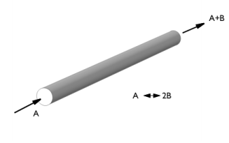
In the New window, Start by adding the individual physics interfaces for mass transfer, fluid flow, and heat transfer in fluids.
2
click  Model Wizard.
Model Wizard
1
In the Model Wizard window, click  2D Axisymmetric.
2
In the Select Physics tree, select Chemical Species Transport > Transport of Concentrated Species (tcs).
3
Click Add.
4
In the Mass fractions (1) table, enter the following settings:
5
In the Select Physics tree, select Fluid Flow > Single-Phase Flow > Laminar Flow (spf).
6
Click Add.
7
In the Select Physics tree, select Heat Transfer > Heat Transfer in Fluids (ht).
8
Click Add.
9
Click  Study.
10
In the Select Study tree, select General Studies > Stationary.
11
Global Definitions
Parameters 1
1
In the Model Builder window, under Global Definitions click Parameters 1.
2
In the Settings window for Parameters, locate the Parameters section.
3
Click  Load from File.
4
Gas System 1 (pp1)
In this model, a Thermodynamic System containing NO2 and N2O4 is used. Import the predefined system from a file. See the Appendix below for details on how to create the system.
1
In the Physics toolbar, click  Thermodynamics and choose Import System.
2
Since NO2 and N2O4 are not available in the built-in thermodynamics database, they have been created as User-Defined Species in the imported file.
Geometry 1
The model geometry is simply a rectangle.
Rectangle 1 (r1)
1
In the Geometry toolbar, click  Rectangle.
2
In the Settings window for Rectangle, locate the Size and Shape section.
3
In the Width text field, type W0.
4
In the Height text field, type L0.
5
Click  Build All Objects.
6
Click the  Zoom Extents button in the Graphics toolbar.
Definitions
Average 1 (aveop1)
1
In the Definitions toolbar, click  Nonlocal Couplings and choose Average.
You will use this function later in the results analysis. With the checkbox Compute integral in revolved geometry enabled, it automatically performs a surface integration by multiplication with 2*pi*r.
2
In the Settings window for Average, locate the Source Selection section.
3
From the Geometric entity level list, choose Boundary.
4
Global Definitions
Use the Gas System 1 to generate a corresponding Chemistry interface.
Gas System 1 (pp1)
In the Model Builder window, under Global Definitions > Thermodynamics right-click Gas System 1 (pp1) and choose Generate Chemistry.
Select Species
1
Go to the Select Species window.
2
Click  Add All.
3
Click the Next button in the window toolbar.
Chemistry Settings
1
Go to the Chemistry Settings window.
2
From the Mass transfer list, choose Concentrated species.
3
Click the Finish button in the window toolbar.
Chemistry (chem)
Reaction 1
1
In the Physics toolbar, click  Domains and choose Reaction.
2
In the Settings window for Reaction, locate the Reaction Formula section.
3
In the Formula text field, type N2O4<=>NO2.
4
Click Apply.
Now, the reaction is unbalanced. To make it stoichiometrically balanced, click Balance.
5
Click Balance in the upper-right corner of the Reaction Formula section.
6
Locate the Rate Constants section. Select the Specify equilibrium constant checkbox.
7
In the kf text field, type kf.
8
In the Model Builder window, click Chemistry (chem).
9
In the Settings window for Chemistry, locate the Species Matching section.
10
Find the Bulk species subsection. From the Species solved for list, choose Transport of Concentrated Species.
11
12
Click to expand the Calculate Transport Properties section. Drag and drop below Materials.
Now add the Reacting Flow multiphysics coupling node. When using the Chemistry interface it supports both isothermal and nonisothermal flow.
Multiphysics
Reacting Flow 1 (nirf1)
In the Physics toolbar, click  Multiphysics Couplings and choose Domain > Reacting Flow.
Laminar Flow (spf)
Since the density variation is large, the flow cannot be regarded as incompressible. Therefore select Compressible flow.
1
In the Model Builder window, under Component 1 (comp1) click Laminar Flow (spf).
2
In the Settings window for Laminar Flow, locate the Physical Model section.
3
From the Compressibility list, choose Compressible flow (Ma<0.3).
Define the pressure reference level in the interface properties.
4
In the pref text field, type p_amb.
Inlet 1
1
In the Physics toolbar, click  Boundaries and choose Inlet.
2
3
In the Settings window for Inlet, locate the Boundary Condition section.
4
From the list, choose Fully developed flow.
5
Locate the Fully Developed Flow section. In the Uav text field, type v_in.
Outlet 1
1
In the Physics toolbar, click  Boundaries and choose Outlet.
2
3
In the Settings window for Outlet, locate the Pressure Conditions section.
4
Select the Normal flow checkbox.
Transport of Concentrated Species (tcs)
1
In the Model Builder window, under Component 1 (comp1) click Transport of Concentrated Species (tcs).
2
In the Settings window for Transport of Concentrated Species, locate the Transport Mechanisms section.
3
From the Diffusion model list, choose Maxwell–Stefan.
4
Locate the Species section. From the From mass constraint list, choose wB.
Species Molar Masses 1
1
In the Model Builder window, under Component 1 (comp1) > Transport of Concentrated Species (tcs) click Species Molar Masses 1.
2
In the Settings window for Species Molar Masses, locate the Molar Mass section.
3
From the MwA list, choose Molar mass (chem/N2O4).
4
From the MwB list, choose Molar mass (chem/NO2).
Fluid 1
1
In the Model Builder window, click Fluid 1.
2
In the Settings window for Fluid, locate the Diffusion section.
3
Reaction Sources 1
1
In the Physics toolbar, click  Domains and choose Reaction Sources.
2
3
In the Settings window for Reaction Sources, locate the Reactions section.
4
From the Chemistry list, choose Chemistry (chem).
Inflow 1
1
In the Physics toolbar, click  Boundaries and choose Inflow.
2
3
In the Settings window for Inflow, locate the Inflow section.
4
In the ω0,wA text field, type wN2O4_in.
Outflow 1
1
In the Physics toolbar, click  Boundaries and choose Outflow.
2
Mesh 1
A mapped mesh is suitable for fluid flow.
Mapped 1
In the Mesh toolbar, click  Mapped.
Distribution 1
1
Right-click Mapped 1 and choose Distribution.
2
3
In the Settings window for Distribution, locate the Distribution section.
4
From the Distribution type list, choose Predefined.
5
In the Number of elements text field, type 100.
6
In the Element ratio text field, type 50.
Distribution 2
1
In the Model Builder window, right-click Mapped 1 and choose Distribution.
2
3
In the Settings window for Distribution, locate the Distribution section.
4
From the Distribution type list, choose Predefined.
5
In the Number of elements text field, type 10.
6
In the Element ratio text field, type 5.
For the isothermal case decouple the Heat Transfer in Fluids interface in the Reacting Flow coupling feature. Also apply a constant value Tf for the temperature. This is needed to provide the reaction rate and density with a valid temperature.
Multiphysics
Reacting Flow 1 (nirf1)
1
In the Model Builder window, under Component 1 (comp1) > Multiphysics click Reacting Flow 1 (nirf1).
2
In the Settings window for Reacting Flow, locate the Coupled Interfaces section.
3
From the Heat transfer (optional, requires Chemistry) list, choose None.
4
Locate the Temperature section. In the T text field, type Tf.
Study - Isothermal Model
1
In the Model Builder window, click Study 1.
2
In the Settings window for Study, type Study - Isothermal Model in the Label text field.
3
Locate the Study Settings section. Clear the Generate default plots checkbox.
Step 1: Stationary
Turn off the Heat Transfer in Fluids interface to avoid solving for the temperature.
1
In the Model Builder window, under Study - Isothermal Model click Step 1: Stationary.
2
In the Settings window for Stationary, locate the Physics and Variables Selection section.
3
In the Solve for column of the table, under Component 1 (comp1), clear the checkbox for Heat Transfer in Fluids (ht).
4
In the Study toolbar, click  Compute.
Results
Global Evaluation 1
1
In the Model Builder window, expand the Results node.
2
Right-click Results > Derived Values and choose Global Evaluation.
3
In the Settings window for Global Evaluation, locate the Expressions section.
4
5
Clicknext to  Evaluate, then choose New Table.
Revolution 2D 1
In the Results toolbar, click  More Datasets and choose Revolution 2D.
Velocity, isothermal
1
In the Results toolbar, click  3D Plot Group.
2
In the Settings window for 3D Plot Group, type Velocity, isothermal in the Label text field.
Multislice 1
1
In the Velocity, isothermal toolbar, click  More Plots and choose Multislice.
2
In the Settings window for Multislice, locate the Expression section.
3
In the Expression text field, type spf.U.
4
Locate the Multiplane Data section. Find the y-planes subsection. In the Planes text field, type 0.
5
Find the z-planes subsection. In the Planes text field, type 10.
6
Locate the Coloring and Style section. From the Color table list, choose Prism.
Mass fraction, B, isothermal
1
In the Model Builder window, right-click Velocity, isothermal and choose Duplicate.
2
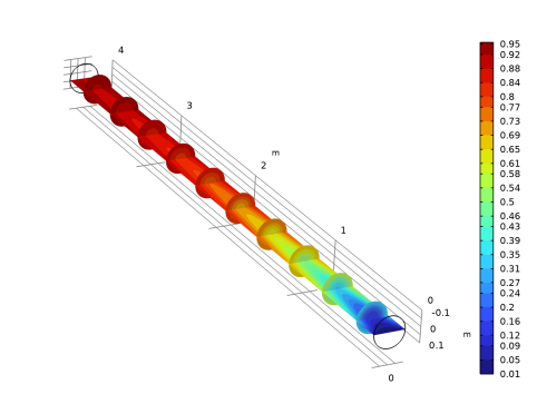
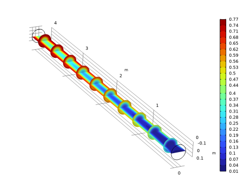
In the Settings window for 3D Plot Group, type Mass fraction, B, isothermal in the Label text field.
Multislice 1
1
In the Model Builder window, expand the Mass fraction, B, isothermal node, then click Multislice 1.
2
In the Settings window for Multislice, click Replace Expression in the upper-right corner of the Expression section. From the menu, choose Component 1 (comp1) > Transport of Concentrated Species > Species wB > wB - Mass fraction, wB - 1.
3
Locate the Coloring and Style section. From the Color table list, choose Rainbow.
4
From the Color table type list, choose Discrete.
5
In the Number of bands text field, type 25.
Add a new study for the nonisothermal simulation. This makes it straightforward to compare results from the two setups.
Add Study
1
In the Home toolbar, click  Add Study to open the Add Study window.
2
Go to the Add Study window.
3
Find the Studies subsection. In the Select Study tree, select General Studies > Stationary.
4
Click the Add Study button in the window toolbar.
5
In the Home toolbar, click  Add Study to close the Add Study window.
Study - Nonisothermal Model
In the Settings window for Study, type Study - Nonisothermal Model in the Label text field.
Now set up the Heat Transfer in Fluids interface. Note that the heat source due to reactions is automatically accounted for when Chemistry is included in the Reacting Flow coupling feature. Hence there is no need to add a Heat Source feature in Heat Transfer in Fluids.
Heat Transfer in Fluids (ht)
Temperature 1
1
In the Physics toolbar, click  Boundaries and choose Temperature.
2
3
In the Settings window for Temperature, locate the Temperature section.
4
In the T0 text field, type T_amb.
Heat Flux 1
1
In the Physics toolbar, click  Boundaries and choose Heat Flux.
2
3
In the Settings window for Heat Flux, locate the Heat Flux section.
4
In the q0 text field, type Ua*(Tf-T).
For the nonisothermal case reenable the Heat Transfer in Fluids interface in the Reacting Flow coupling feature. This synchronizes the temperature solved for among all other coupled interfaces. The thermodynamic properties of the mixture are defined by the Chemistry interface.
Multiphysics
Reacting Flow 1 (nirf1)
1
In the Model Builder window, under Component 1 (comp1) > Multiphysics click Reacting Flow 1 (nirf1).
2
In the Settings window for Reacting Flow, locate the Coupled Interfaces section.
3
From the Heat transfer (optional, requires Chemistry) list, choose Heat Transfer in Fluids (ht).
Study - Nonisothermal Model
1
In the Model Builder window, click Study - Nonisothermal Model.
2
In the Settings window for Study, locate the Study Settings section.
3
Clear the Generate default plots checkbox.
4
In the Study toolbar, click  Compute.
Results
Global Evaluation 2
1
In the Model Builder window, under Results > Derived Values right-click Global Evaluation 1 and choose Duplicate.
2
In the Settings window for Global Evaluation, locate the Data section.
3
From the Dataset list, choose Study - Nonisothermal Model/Solution 2 (sol2).
4
Clicknext to  Evaluate, then choose Table 1 - Global Evaluation 1.
Revolution 2D 2
1
In the Results toolbar, click  More Datasets and choose Revolution 2D.
2
In the Settings window for Revolution 2D, locate the Data section.
3
From the Dataset list, choose Study - Nonisothermal Model/Solution 2 (sol2).
Velocity, nonisothermal
1
In the Model Builder window, right-click Velocity, isothermal and choose Duplicate.
2
In the Settings window for 3D Plot Group, type Velocity, nonisothermal in the Label text field.
3
Locate the Data section. From the Dataset list, choose Revolution 2D 2.
4
Locate the Plot Settings section. From the View list, choose View 3D 2.
Mass fraction B, nonisothermal
1
In the Model Builder window, expand the Velocity, nonisothermal node.
2
Right-click Mass fraction, B, isothermal and choose Duplicate.
3
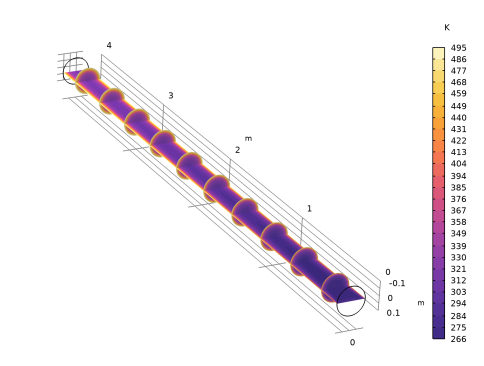
In the Settings window for 3D Plot Group, type Mass fraction B, nonisothermal in the Label text field.
4
Locate the Data section. From the Dataset list, choose Revolution 2D 2.
5
Locate the Plot Settings section. From the View list, choose View 3D 2.
6
In the Mass fraction B, nonisothermal toolbar, click  Plot.
7
Click the  Zoom Extents button in the Graphics toolbar.
Temperature
1
Right-click Mass fraction B, nonisothermal and choose Duplicate.
2
In the Settings window for 3D Plot Group, type Temperature in the Label text field.
3
In the Temperature toolbar, click  Plot.
Multislice 1
1
In the Model Builder window, expand the Temperature node, then click Multislice 1.
2
In the Settings window for Multislice, click Replace Expression in the upper-right corner of the Expression section. From the menu, choose Component 1 (comp1) > Heat Transfer in Fluids > Temperature > T - Temperature - K.
3
Locate the Coloring and Style section. From the Color table list, choose HeatCameraLight.
4
In the Temperature toolbar, click  Plot.
5
Click the  Zoom Extents button in the Graphics toolbar.
Appendix
Follow the steps below to create the thermodynamic system used in the model. Two User-Defined Species are also created.
From the File menu, choose New.
New
In the New window, click  Blank Model.
Global Definitions
In the Physics toolbar, click  Thermodynamics and choose User-Defined Species.
Enter Name and Formula
1
Go to the Enter Name and Formula window.
2
3
4
5
Click the Next button in the window toolbar.
Enter Parameters
1
Go to the Enter Parameters window.
2
Find the Constants subsection. In the table, enter the following settings:
3
Find the Model parameters subsection. In the table, enter the following settings:
4
Click the Next button in the window toolbar.
Define Properties
1
Go to the Define Properties window.
2
Find the Heat capacity (J/(K*mol)) subsection. Click  Add.
3
In the Ideal gas table, enter the following settings:
4
5
In the Ideal gas table, enter the following settings:
6
7
In the Ideal gas table, enter the following settings:
8
9
In the Ideal gas table, enter the following settings:
10
11
In the Ideal gas table, enter the following settings:
12
13
In the Ideal gas table, enter the following settings:
14
Find the Saturated liquid density (mol/m^3) subsection. In the Natural logarithm liquid viscosity table, enter the following settings:
15
Find the Thermal conductivity (W/(K*m)) subsection. Click  Add.
16
In the Vapor table, enter the following settings:
17
Find the Vapor viscosity (Pa*s) subsection. Click  Add.
18
In the Vapor viscosity table, enter the following settings:
19
20
In the Vapor viscosity table, enter the following settings:
21
22
In the Vapor viscosity table, enter the following settings:
23
Click the Finish button in the window toolbar.
Define species NO2.
Global Definitions
In the Physics toolbar, click  Thermodynamics and choose User-Defined Species.
Enter Name and Formula
1
Go to the Enter Name and Formula window.
2
3
4
5
Click the Next button in the window toolbar.
Enter Parameters
1
Go to the Enter Parameters window.
2
Find the Constants subsection. In the table, enter the following settings:
3
Find the Model parameters subsection. In the table, enter the following settings:
4
Click the Next button in the window toolbar.
Define Properties
1
Go to the Define Properties window.
2
Find the Heat capacity (J/(K*mol)) subsection. Click  Add.
3
In the Ideal gas table, enter the following settings:
4
5
In the Ideal gas table, enter the following settings:
6
7
In the Ideal gas table, enter the following settings:
8
9
In the Ideal gas table, enter the following settings:
10
Find the Saturated liquid density (mol/m^3) subsection. In the Natural logarithm liquid viscosity table, enter the following settings:
11
12
In the Natural logarithm liquid viscosity table, enter the following settings:
13
14
In the Natural logarithm liquid viscosity table, enter the following settings:
15
16
In the Natural logarithm liquid viscosity table, enter the following settings:
17
18
In the Natural logarithm liquid viscosity table, enter the following settings:
19
20
In the Natural logarithm liquid viscosity table, enter the following settings:
21
22
In the Natural logarithm liquid viscosity table, enter the following settings:
23
24
In the Natural logarithm liquid viscosity table, enter the following settings:
25
26
In the Natural logarithm liquid viscosity table, enter the following settings:
27
28
In the Natural logarithm liquid viscosity table, enter the following settings:
29
30
In the Natural logarithm liquid viscosity table, enter the following settings:
31
Find the Thermal conductivity (W/(K*m)) subsection. Click  Add.
32
In the Vapor table, enter the following settings:
33
34
In the Vapor table, enter the following settings:
35
36
In the Vapor table, enter the following settings:
37
38
In the Vapor table, enter the following settings:
39
40
In the Vapor table, enter the following settings:
41
42
In the Vapor table, enter the following settings:
43
44
In the Vapor table, enter the following settings:
45
Find the Vapor viscosity (Pa*s) subsection. Click  Add.
46
In the Vapor viscosity table, enter the following settings:
47
48
In the Vapor viscosity table, enter the following settings:
49
50
In the Vapor viscosity table, enter the following settings:
51
52
In the Vapor viscosity table, enter the following settings:
53
54
In the Vapor viscosity table, enter the following settings:
55
56
In the Vapor viscosity table, enter the following settings:
57
Click the Finish button in the window toolbar.
Create a Thermodynamic System including the created species.
Global Definitions
In the Physics toolbar, click  Thermodynamics and choose Thermodynamic System.
Select System
1
Go to the Select System window.
2
Click the Next button in the window toolbar.
Select Species
1
Go to the Select Species window.
2
From the Database list, choose User defined.
3
Click  Add All.
4
Click the Next button in the window toolbar.
Select Thermodynamic Model
1
Go to the Select Thermodynamic Model window.
2
Click the Finish button in the window toolbar.
Global Definitions
Gas System 1 (pp1)
1
Right-click Global Definitions > Thermodynamics > Gas System 1 (pp1) and choose Export Thermodynamic System.
2
Browse to a suitable folder, enter the filename dissociation_thermo_system.xml, and then click Save.