PDF

Multiobjective Optimization of Paracetamol Cooling Crystallization
Introduction
Cooling crystallization is a common separation process in many fields where crystal properties such as crystal size and crystal shape are important. To get the desired end product, the cooling curve can be programmatically predefined.
This example model shows the multiobjective optimization of a cooling curve used for the unseeded batch crystallization of paracetamol in ethanol. The model uses Efficient Global Optimization (EGO) to maximize yield within a specified size range and minimize the number of small crystals.
Model Definition
The crystallization is assumed to occur in a perfectly mixed reactor and is thus modeled in 0D. The crystallization process is modeled with the Size-Based Population Balance interface across a size range of 1 nm to 1000 μm. The size range is discretized logarithmically using 100 intervals. A logarithmic distribution is suitable when nucleation is included. For the crystals, a volume shape factor, kv, of 0.797 is used (Ref. 1).
Crystal nucleation is modeled according to (Ref. 1)
(1)
and
(2)
where Kb,1 and Kb,2 are the primary and secondary nucleation rate constants (1/m3/s), νmol is the solute molecule volume (m3), ms is the mass fraction of solid particles (kg/kg), σ is the interfacial energy (J/m2), while α and β are dimensionless constants. The solute molecule volume is estimated from its solid form density and molar mass. The growth and dissolution rates are modeled according to (Ref. 1)
(3)
and
(4)
where Kg and Kd are the growth and dissolution rate constants (m/s) and Eag and Ead are the growth and dissolution rate activation energies (J/mol). The dissolution rate is defined such that it assumes a negative value. The Size-Based Population Balance interface expects a negative dissolution rate. In the above equations, S (-) and ΔC (g/g) are measures of the supersaturation defined as
(5)
(6)
where C is the paracetamol concentration (g/g) and C* is the paracetamol solubility as a function of temperature (g/g). The parameter values in equations 1-4 are taken from Ref. 1.
The temperature, T, follows a parameterized cooling curve consisting of a constant temperature region followed by a temperature cycling region, similar to what was done in Ref. 1. The constant temperature region is typically where most of the crystal mass is formed while the temperature cycling region typically provides an opportunity to dissolve small crystals. Cooling takes place across 350 minutes starting at 50°C and ending at 20°C. The curve shape depends on five parameter values. The p parameter controls the height of the initial plateau temperature while the parameters a, b, c, and d control the height of subsequent peaks in the temperature cycling region. The constant plateau temperature can vary between 20 and 45°C while each individual peak height can vary between 0 and 10°C.
Figure 1: Cooling curve with optimization parameters.
The optimization objective for the model was based on maximizing yield within a specified size range (145–330 μm) and minimize the number of small crystals (145 μm). The objective function to be maximized can be written as the sum of three separate objective functions
(7)
The objective function assumes a value between 0 and 1. The separate objective functions describe the normalized volume concentration of target particles
(8),
the mass of target particles normalized by the theoretical maximum mass
(9),
and the number fraction of particles smaller than the target particles
(10)
In the above objective functions, n is the continuous number density distribution (1/m4), L is the particle size (m), ρp is the solid crystal particle density (kg/m3), ρsol is the solvent density (kg/m3), and C0 is the initial concentration (g/g). The sizes L1 and L2 equal 145 and 330 μm respectively.
Results and Discussion
Figure 2 shows the cooling curve for five different cases from the optimization process. The color legend shows the total objective score for each case and the solid line is the optimized case. The objective score of the optimal solution (solid line) was 0.68 and the cooling curve had a plateau at 30.5°C followed by one large and two smaller peaks in the temperature cycling region.
Figure 2: Cooling curves for different cases. The optimized case is shown with a solid line.
The corresponding supersaturation curves can be seen in Figure 3. The supersaturation curve for the optimized case ends near the saturation line (S=1) giving a high product yield.
Figure 3: Supersaturation curves for different cases. The optimized case is shown with a solid line.
The volume density distribution for the same cases as in the two previous figures can be seen in Figure 4. It shows that cooling curves that have a higher initial plateau, leading to an overall slower cooling rate, result in wider distributions. For the cases marked with asterisks, two distinct bumps can be seen in the distribution. This is caused by undersaturation at 170 minutes prompting dissolution and creating a divide in the distribution. When investigating the cooling curves, it can be seen that this corresponds to the first peak in the cycling region. As there is a high temperature plateau, the solution is close to the saturation point before the first temperature cycle, causing undersaturation.
Figure 4: Volume density distributions for different cases. The optimized case is shown with a solid line.
The concentration and solubility for the optimized case can be seen in Figure 5.
Figure 5: Concentration and solubility for the optimized case.
Figure 6 shows the growth/dissolution rate of crystals for the optimized case. The time interval where crystals are dissolving aligns with where the concentration is below the solubility in Figure 5.
Figure 6: Growth/dissolution rate for the optimized case.
Reference
1. Y. Kim, Y. Kawajiri, R.W. Rousseau, and M.A. Grover, “Modeling of Nucleation, Growth, and Dissolution of Paracetamol in Ethanol Solution for Unseeded Batch Cooling Crystallization with Temperature-Cycling Strategy,” Ind. Eng. Chem. Res., vol. 62, no. 6, pp. 2866-2881, 2017; Copyright 2023 The Authors. Published by American Chemical Society. This publication is licensed under CC-BY 4.0.
Application Library path: Chemical_Reaction_Engineering_Module/Mixing_and_Separation/cooling_crystallization_optimization
Modeling Instructions
From the File menu, choose New.
New
In the New window, click  Model Wizard.
Model Wizard
1
In the Model Wizard window, click  0D.
2
In the Select Physics tree, select Chemical Species Transport > Precipitation and Crystallization > Precipitation and Crystallization.
3
Click Add.
4
Click  Study.
5
In the Select Study tree, select General Studies > Time Dependent.
6
Global Definitions
Parameters 1
1
In the Model Builder window, under Global Definitions click Parameters 1.
2
In the Settings window for Parameters, locate the Parameters section.
3
Click  Load from File.
4
Definitions
Variables 1
1
In the Definitions toolbar, click  Local Variables.
2
In the Settings window for Variables, locate the Variables section.
3
Click  Load from File.
4
Solubility Curve
1
In the Home toolbar, click  Functions and choose Local > Analytic.
2
In the Settings window for Analytic, type Solubility Curve in the Label text field.
3
In the Function name text field, type sol.
4
Locate the Definition section. In the Expression text field, type -8.707+9.669*1e-2*T-3.610*1e-4*T^2+4.590*1e-7*T^3.
5
In the Arguments text field, type T.
6
Locate the Units section. In the Function text field, type g/g.
7
Cooling Curve
1
In the Home toolbar, click  Functions and choose Local > Interpolation.
2
In the Settings window for Interpolation, type Cooling Curve in the Label text field.
3
Locate the Definition section. In the Function name text field, type temp.
4
Click  Load from File.
5
Browse to the model’s Application Libraries folder and double-click the file cooling_crystallization_optimization_cooling_curve.txt.
6
Locate the Interpolation and Extrapolation section. From the Extrapolation list, choose Linear.
7
Locate the Units section. In the Function table, enter the following settings:
8
In the Argument table, enter the following settings:
The imported cooling curve depends on five parameters, a, b, c, d, and p. The first four control the temperature cycling in the second half of the process, while the fifth controls the plateau temperature in the first half.
Reaction Engineering (re)
1
In the Model Builder window, under Component 1 (comp1) click Reaction Engineering (re).
2
In the Settings window for Reaction Engineering, locate the Energy Balance section.
3
In the T text field, type temp(t).
4
Locate the Mixture Properties section. From the Phase list, choose Liquid.
Species 1
1
In the Reaction Engineering toolbar, click  Species.
2
In the Settings window for Species, locate the Name section.
3
Initial Values 1
1
In the Model Builder window, click Initial Values 1.
2
In the Settings window for Initial Values, locate the Volumetric Species Initial Values section.
3
Size-Based Population Balance (pbsb)
1
In the Model Builder window, under Component 1 (comp1) click Size-Based Population Balance (pbsb).
2
In the Settings window for Size-Based Population Balance, locate the Particle Properties section.
3
In the ρp text field, type rho_p.
4
From the Particle shape list, choose User defined. In the ka text field, type 1.
5
In the kv text field, type 0.797.
6
Locate the Size Intervals section. From the Discretization list, choose Logarithmic.
7
In the I text field, type 100.
8
In the L0 text field, type 1[nm].
9
In the LI text field, type 1000[µm].
10
Locate the Nucleation section. In the Bnuc text field, type if(S>1,kb2*(S-1+eps)^alpha*ms^(beta),0)+if(S>1,kb*exp(-(16*pi*v_mol^2*sig^3)/(3*k_B_const^3*T^3*(log(S))^2)),0).
11
Locate the Growth and Dissolution section. In the GL text field, type if(DeltaC>0,kg*exp(-Eag/(R_const*T))*DeltaC^gamma_g,0).
12
In the DL text field, type if(DeltaC<0,-kd*exp(-Ead/(R_const*T))*(-DeltaC)^gamma_d,0).
1
In the Model Builder window, under Component 1 (comp1) > Size-Based Population Balance (pbsb) click Initial Values 1.
2
In the Settings window for Initial Values, locate the Population Number Density section.
3
In the n0 text field, type 1.
Study 1
Parameter Optimization
1
In the Study toolbar, click  Optimization and choose Parameter Optimization.
2
In the Settings window for Parameter Optimization, locate the Optimization Solver section.
3
From the Method list, choose EGO.
4
Locate the Objective Function section. In the table, enter the following settings:
5
From the Type list, choose Maximization.
6
From the Solution list, choose Use last.
7
Locate the Control Parameters section. Click  Add.
8
9
10
11
12
13
14
15
16
17
Click to expand the Output section. From the Keep solutions list, choose All.
Step 1: Time Dependent
1
In the Model Builder window, click Step 1: Time Dependent.
2
In the Settings window for Time Dependent, locate the Study Settings section.
3
In the Output times text field, type range(0,0.5[min],tf).
Solution 1 (sol1)
1
In the Study toolbar, click  Show Default Solver.
2
In the Model Builder window, expand the Solution 1 (sol1) node, then click Time-Dependent Solver 1.
3
In the Settings window for Time-Dependent Solver, locate the General section.
4
In the Store every Nth step text field, type 50.
5
In the Study toolbar, click  Compute.
Results
1
In the Model Builder window, click Results.
2
In the Settings window for Results, locate the Update of Results section.
3
Select the Only plot when requested checkbox.
Preferred Units 1
1
In the Results toolbar, click  Configurations and choose Preferred Units.
2
In the Settings window for Preferred Units, locate the Units section.
3
Click  Add Physical Quantity.
4
In the Physical Quantity dialog, type len in the text field.
5
In the tree, select General > Length (m).
6
7
In the Settings window for Preferred Units, locate the Units section.
8
Concentration and Solubility
1
In the Model Builder window, under Results click Concentration (re).
2
In the Settings window for 1D Plot Group, locate the Data section.
3
From the Parameter selection (p, a, b, c, d) list, choose Last.
4
In the Label text field, type Concentration and Solubility.
5
Locate the Plot Settings section.
6
Select the y-axis label checkbox. In the associated text field, type Concentration (g/g).
Global 1
1
In the Model Builder window, expand the Concentration and Solubility node, then click Global 1.
2
In the Settings window for Global, locate the y-Axis Data section.
3
4
Locate the x-Axis Data section. From the Unit list, choose min.
5
Click to expand the Coloring and Style section. From the Width list, choose 2.
6
Click to expand the Legends section. Find the Include subsection. Clear the Solution checkbox.
7
Clear the Expression checkbox.
8
Select the Description checkbox.
Concentration and Solubility
In the Concentration and Solubility toolbar, click  Line Segments.
Line Segments 1
1
In the Settings window for Line Segments, locate the x-Coordinates section.
2
3
Locate the y-Coordinates section. In the table, enter the following settings:
4
Click to expand the Coloring and Style section. Find the Line style subsection. From the Line list, choose Dotted.
5
From the Color list, choose Red.
Concentration and Solubility
In the Concentration and Solubility toolbar, click  Annotation.
Annotation 1
1
In the Settings window for Annotation, locate the Annotation section.
2
In the Text text field, type Supersaturation.
3
Locate the Position section. In the x text field, type 42.
4
In the y text field, type (at(42[min], C)+at(42[min], sol(T)))/2.
5
Locate the Coloring and Style section. Clear the Show point checkbox.
6
From the Anchor point list, choose Lower middle.
7
From the Orientation list, choose Vertical.
8
In the Concentration and Solubility toolbar, click  Plot.
Average Size Distribution (pbsb)
1
In the Model Builder window, under Results click Average Size Distribution (pbsb).
2
In the Settings window for 1D Plot Group, locate the Data section.
3
From the Time selection list, choose Last.
4
From the Parameter selection (p, a, b, c, d) list, choose Last.
5
In the Average Size Distribution (pbsb) toolbar, click  Plot.
Result Templates
1
In the Results toolbar, click  Result Templates to open the Result Templates window.
2
Go to the Result Templates window.
3
In the tree, select Study 1/Parametric Solutions 1 (sol2) > Size-Based Population Balance > Volume Density Distribution (pbsb).
4
Click the Add Result Template button in the window toolbar.
5
In the Results toolbar, click  Result Templates to close the Result Templates window.
Results
Volume Density Distribution (pbsb)
1
In the Settings window for 1D Plot Group, locate the Data section.
2
From the Parameter selection (p, a, b, c, d) list, choose Last.
3
From the Time selection list, choose Last.
4
Locate the Plot Settings section. In the x-axis label text field, type Size (µm).
Line Segments 1
1
In the Model Builder window, expand the Volume Density Distribution (pbsb) node, then click Line Segments 1.
2
In the Settings window for Line Segments, locate the Coloring and Style section.
3
From the Color list, choose Black.
4
From the Width list, choose 2.
Volume Density Distribution (pbsb)
In the Volume Density Distribution (pbsb) toolbar, click  Line Segments.
Line Segments 2
1
In the Settings window for Line Segments, locate the x-Coordinates section.
2
3
Locate the y-Coordinates section. In the table, enter the following settings:
4
Locate the Coloring and Style section. Find the Line style subsection. From the Line list, choose Dotted.
5
From the Color list, choose Red.
6
From the Width list, choose 2.
Line Segments 3
1
Right-click Results > Volume Density Distribution (pbsb) > Line Segments 2 and choose Duplicate.
2
In the Settings window for Line Segments, locate the x-Coordinates section.
3
Volume Density Distribution (pbsb)
In the Volume Density Distribution (pbsb) toolbar, click  Annotation.
Annotation 1
1
In the Settings window for Annotation, locate the Annotation section.
2
In the Text text field, type \textbf{\unicode{?}} Volume fraction of particles in target area = eval(TVf) \\ \\ \textbf{\unicode{?}} Crystal mass fraction of theoretical max in target area = eval(Vf) \\ \\ \textbf{\unicode{?}} Number fraction of particles below the target area = eval(N_small) \\ \\ Total maximization objective score (0-1) = eval(Vf/4+TVf/4+(1-N_small)/2).
3
Select the LaTeX markup checkbox.
4
Locate the Position section. In the x text field, type 700.
5
In the y text field, type 200.
6
Locate the Coloring and Style section. Clear the Show point checkbox.
7
From the Anchor point list, choose Center.
8
In the Volume Density Distribution (pbsb) toolbar, click  Plot.
Growth and Dissolution
1
In the Results toolbar, click  1D Plot Group.
2
In the Settings window for 1D Plot Group, type Growth and Dissolution in the Label text field.
3
Click to expand the Title section. From the Title type list, choose None.
4
Locate the Plot Settings section.
5
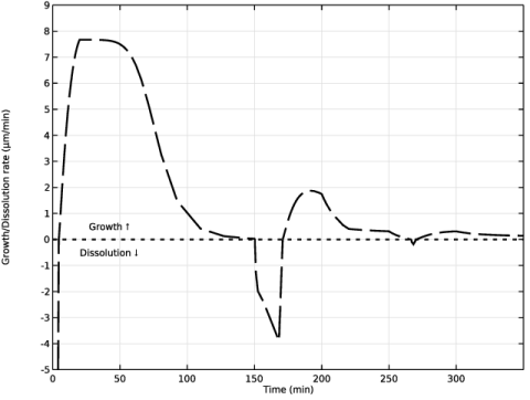
Select the y-axis label checkbox. In the associated text field, type Growth/Dissolution rate (µm/min).
6
Locate the Axis section. Select the Manual axis limits checkbox.
7
In the x minimum text field, type 0.
8
In the x maximum text field, type tf/60.
9
In the y minimum text field, type -5.
10
In the y maximum text field, type 9.
11
Locate the Legend section. Clear the Show legends checkbox.
Global 1
1
In the Growth and Dissolution toolbar, click  Global.
2
In the Settings window for Global, locate the y-Axis Data section.
3
4
Locate the x-Axis Data section. From the Unit list, choose min.
5
Locate the Coloring and Style section. Find the Line style subsection. From the Line list, choose Dashed.
6
From the Color list, choose Black.
7
From the Width list, choose 2.
Growth and Dissolution
In the Growth and Dissolution toolbar, click  Global.
Global 2
1
In the Settings window for Global, locate the y-Axis Data section.
2
3
Locate the x-Axis Data section. From the Unit list, choose min.
4
Locate the Coloring and Style section. Find the Line style subsection. From the Line list, choose Dotted.
5
From the Color list, choose Black.
6
From the Width list, choose 2.
Growth and Dissolution
In the Growth and Dissolution toolbar, click  Annotation.
Annotation 1
1
In the Settings window for Annotation, locate the Annotation section.
2
In the Text text field, type Growth ?.
3
Locate the Position section. In the x text field, type 42.
4
In the y text field, type 0.5.
5
Locate the Coloring and Style section. Clear the Show point checkbox.
6
From the Anchor point list, choose Center.
Annotation 2
1
Right-click Results > Growth and Dissolution > Annotation 1 and choose Duplicate.
2
In the Settings window for Annotation, locate the Annotation section.
3
In the Text text field, type Dissolution ?.
4
Locate the Position section. In the y text field, type -0.5.
5
In the Growth and Dissolution toolbar, click  Plot.
Cooling Curve
1
In the Home toolbar, click  Add Plot Group and choose 1D Plot Group.
2
In the Settings window for 1D Plot Group, type Cooling Curve in the Label text field.
3
Locate the Data section. From the Dataset list, choose Study 1/Parametric Solutions 1 (sol2).
4
From the Parameter selection (p, a, b, c, d) list, choose Manual.
5
In the Parameter indices (1-62) text field, type 1,19,27,46.
6
Locate the Title section. From the Title type list, choose None.
7
Locate the Plot Settings section.
8
Select the y-axis label checkbox. In the associated text field, type Temperature (°C).
Global 1
1
In the Cooling Curve toolbar, click  Global.
2
In the Settings window for Global, locate the y-Axis Data section.
3
4
Locate the x-Axis Data section. From the Unit list, choose min.
5
Locate the Coloring and Style section. Find the Line style subsection. From the Line list, choose Dotted.
6
From the Width list, choose 2.
7
Find the Line markers subsection. From the Marker list, choose Cycle.
8
From the Positioning list, choose Interpolated.
9
In the Number text field, type 10.
10
Locate the Legends section. Clear the Show legends checkbox.
Color Expression 1
1
In the Cooling Curve toolbar, click  Color Expression.
2
In the Settings window for Color Expression, locate the Expression section.
3
In the Expression text field, type at(tf, (1-comp1.N_small)/2+comp1.TVf/4+comp1.Vf/4).
4
Locate the Coloring and Style section. From the Color table list, choose Agama.
5
Click to expand the Range section. Select the Manual color range checkbox.
6
In the Maximum text field, type 0.68465.
7
Locate the Coloring and Style section. From the Color table transformation list, choose Nonlinear.
8
In the Color calibration parameter text field, type 1.
Cooling Curve
1
In the Model Builder window, under Results click Cooling Curve.
2
In the Settings window for 1D Plot Group, locate the Color Legend section.
3
Select the Show titles checkbox.
Color Expression 1
1
In the Model Builder window, under Results > Cooling Curve > Global 1 click Color Expression 1.
2
In the Settings window for Color Expression, locate the Coloring and Style section.
3
In the Color legend title text field, type Objective.
Cooling Curve
In the Cooling Curve toolbar, click  Global.
Global 2
1
In the Settings window for Global, locate the Data section.
2
From the Dataset list, choose Study 1/Solution 1 (sol1).
3
Locate the y-Axis Data section. In the table, enter the following settings:
4
Locate the x-Axis Data section. From the Unit list, choose min.
5
Locate the Coloring and Style section. From the Color list, choose Color table.
6
From the Color table list, choose Agama.
7
Select the Reverse color table checkbox.
8
From the Length of cycle list, choose Manual.
9
In the Number of colors text field, type 2.
10
From the Width list, choose 3.
11
Locate the Legends section. Clear the Show legends checkbox.
12
In the Cooling Curve toolbar, click  Plot.
Supersaturation
1
In the Model Builder window, right-click Cooling Curve and choose Duplicate.
2
In the Settings window for 1D Plot Group, type Supersaturation in the Label text field.
3
Locate the Plot Settings section. In the y-axis label text field, type Supersaturation (1).
Global 1
1
In the Model Builder window, expand the Supersaturation node, then click Global 1.
2
In the Settings window for Global, locate the y-Axis Data section.
3
Global 2
1
In the Model Builder window, click Global 2.
2
In the Settings window for Global, locate the y-Axis Data section.
3
4
In the Supersaturation toolbar, click  Plot.