|
|
|

|
9.92·10-4
|
||||
|
1.00·10-2
|
||||
|
1
|
|
2
|
|
3
|
Click Add.
|
|
4
|
Click
|
|
5
|
|
6
|
Click
|
|
1
|
|
2
|
|
3
|
Click
|
|
4
|
Browse to the model’s Application Libraries folder and double-click the file beer_fermentation_parameters.txt.
|
|
1
|
In the Model Builder window, under Component 1 (comp1) right-click Definitions and choose Variables.
|
|
2
|
|
3
|
Click
|
|
4
|
Browse to the model’s Application Libraries folder and double-click the file beer_fermentation_variables.txt.
|
|
1
|
|
2
|
|
3
|
|
4
|
|
5
|
|
1
|
|
2
|
|
4
|
|
5
|
|
1
|
|
2
|
|
3
|
|
4
|
|
5
|
|
6
|
Locate the Reaction Thermodynamic Properties section. From the Enthalpy of reaction list, choose User defined.
|
|
7
|
|
1
|
|
2
|
|
3
|
Select the Enable formula checkbox.
|
|
4
|
In the text field, type C2H5OH.
|
|
5
|
|
6
|
|
1
|
|
2
|
|
3
|
From the list, choose User defined.
|
|
4
|
|
1
|
|
2
|
|
3
|
Select the Enable formula checkbox.
|
|
4
|
In the text field, type C4H8O2.
|
|
5
|
|
6
|
|
1
|
|
2
|
|
3
|
Select the Enable formula checkbox.
|
|
4
|
In the text field, type C2H4O.
|
|
5
|
|
6
|
|
1
|
|
2
|
|
3
|
|
4
|
Click Apply.
|
|
5
|
|
6
|
|
7
|
Locate the Reaction Thermodynamic Properties section. From the Enthalpy of reaction list, choose User defined.
|
|
8
|
|
1
|
|
2
|
|
3
|
|
4
|
Click Apply.
|
|
5
|
|
6
|
|
7
|
Locate the Reaction Thermodynamic Properties section. From the Enthalpy of reaction list, choose User defined.
|
|
8
|
|
1
|
|
2
|
|
3
|
Clear the Enable formula checkbox.
|
|
1
|
|
2
|
|
3
|
|
4
|
|
5
|
|
6
|
|
7
|
|
1
|
|
2
|
In the text field, type CO2(g).
|
|
3
|
|
4
|
|
1
|
|
2
|
|
3
|
|
4
|
Locate the Volumetric Species Initial Values section. In the table, enter the following settings:
|
|
1
|
|
2
|
|
3
|
|
4
|
|
5
|
|
6
|
|
1
|
|
2
|
|
3
|
|
4
|
|
5
|
|
6
|
Click
|
|
1
|
|
1
|
|
2
|
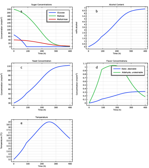
In the Settings window for Global, click Replace Expression in the upper-right corner of the y-Axis Data section. From the menu, choose Component 1 (comp1) > Reaction Engineering > re.c_G - Concentration - mol/m³.
|
|
3
|
Click Add Expression in the upper-right corner of the y-Axis Data section. From the menu, choose Component 1 (comp1) > Reaction Engineering > re.c_M - Concentration - mol/m³.
|
|
4
|
Click Add Expression in the upper-right corner of the y-Axis Data section. From the menu, choose Component 1 (comp1) > Reaction Engineering > re.c_N - Concentration - mol/m³.
|
|
5
|
|
6
|
|
7
|
|
8
|
|
10
|
|
1
|
|
2
|
|
3
|
Locate the Plot Settings section.
|
|
4
|
|
1
|
|
2
|
In the Settings window for Global, click Replace Expression in the upper-right corner of the y-Axis Data section. From the menu, choose Component 1 (comp1) > Definitions > Variables > Evol - vol% alcohol - 1.
|
|
3
|
|
4
|
|
5
|
|
1
|
|
2
|
|
3
|
Locate the Plot Settings section. In the y-axis label text field, type Concentration (mol/m<sup>3</sup>).
|
|
1
|
|
2
|
In the Settings window for Global, click Replace Expression in the upper-right corner of the y-Axis Data section. From the menu, choose Component 1 (comp1) > Reaction Engineering > re.c_X - Concentration - mol/m³.
|
|
3
|
|
4
|
|
1
|
|
2
|
|
1
|
|
2
|
In the Settings window for Global, click Replace Expression in the upper-right corner of the y-Axis Data section. From the menu, choose Component 1 (comp1) > Reaction Engineering > re.c_EtAc - Concentration - mol/m³.
|
|
3
|
Click Add Expression in the upper-right corner of the y-Axis Data section. From the menu, choose Component 1 (comp1) > Reaction Engineering > re.c_AcA - Concentration - mol/m³.
|
|
4
|
|
5
|
Locate the Legends section. In the table, enter the following settings:
|
|
6
|
|
1
|
|
2
|
|
3
|
|
1
|
|
2
|
|
4
|
|
5
|
|
6
|
|
7
|
|
8
|