PDF

Finding Kinetic Arrhenius Parameters Using Parameter Estimation
Introduction
This example shows how to use the Parameter Estimation global feature and the Reaction Engineering interface to find the Arrhenius parameters of a first order reaction. Inspiration for this example is taken from Ref. 1.
Model Definition
Benzene diazonium chloride in the gas phase decomposes to benzene chloride and nitrogen according to
The reaction is first order with the rate:
where the temperature dependent rate constant given by
Above, A is the frequency factor (SI unit: 1/s) and E is the activation energy (SI unit: J/mol).
In order to evaluate the Arrhenius parameters, A and E, a set of experiments was conducted using a perfectly mixed isothermal batch system with constant volume. The concentration of benzene diazonium chloride was monitored as function of time for the temperatures; T = 313 K, 319 K, 323 K, 328 K, and 333 K.
The model optimizes A and E at these temperatures with the Parameter Estimation feature for simulations utilizing the isothermal constant volume Batch reactor type. Five experimental datasets are available in the model file as comma-separated value files (csv-files).
Results and Discussion
Parameter estimation calculations give the values A = 1.17·1016 (SI unit: 1/s) and E = 116 (SI unit: kJ/mol) for the frequency factor and activation energy, respectively. Figure 1 plots the model results and the associated experimental data points.
Figure 1: Model results and experimental data for PhN2Cl concentration as a function of time.
Notes About the COMSOL Implementation
The parameter estimation solver is more efficient in finding an optimal parameter set if the model experiences similar sensitivity with respect to changes in parameter values. In this problem a parameter Aex is therefore defined, that is to be estimated together with the activation energy, E, such that the rate constant is written as:
The frequency factor A is then evaluated as:
The data indicates that the rate constant is of the order ~1·10-3 (1/s) at T = 323 K. Taking this into account and using an initial guess for the activation energy of 150 kJ/mol, an initial guess is set for Aex = 49.
Reference
1. H.S. Fogler, Elements of Chemical Reaction Engineering, 4th ed., p. 95, Prentice Hall, 2005.
Application Library path: Chemical_Reaction_Engineering_Module/Tutorials/activation_energy
Modeling Instructions
From the File menu, choose New.
New
In the New window, click  Model Wizard.
Model Wizard
1
In the Model Wizard window, click  0D.
2
In the Select Physics tree, select Chemical Species Transport > Reaction Engineering (re).
3
Click Add.
4
Click  Study.
5
In the Select Study tree, select General Studies > Time Dependent.
6
Global Definitions
Add a set of model parameters by importing their definitions from a data text file.
Parameters 1
1
In the Model Builder window, under Global Definitions click Parameters 1.
2
In the Settings window for Parameters, locate the Parameters section.
3
Click  Load from File.
4
Alternatively, type in the parameters directly in the Parameters section.
Reaction Engineering (re)
Define the parameter T_iso.
1
In the Model Builder window, under Component 1 (comp1) click Reaction Engineering (re).
2
In the Settings window for Reaction Engineering, locate the Energy Balance section.
3
In the T text field, type T_iso.
The reaction formula, as well as initial values for the chemical components, are added in the following way.
Reaction 1
1
In the Reaction Engineering toolbar, click  Reaction.
2
In the Settings window for Reaction, locate the Reaction Formula section.
3
In the Formula text field, type PhN2Cl=>PhCl+N2.
Initial Values 1
1
In the Model Builder window, click Initial Values 1.
2
In the Settings window for Initial Values, locate the Volumetric Species Initial Values section.
3
Now, add a Parameter Estimation feature and define the global least-squares objectives to be used during optimization. Add one Least-Squares Objective node for each set of experimental data available. In this tutorial model there are data from five different experiments.
Component 1 (comp1)
Experimental data 313 K
1
In the Model Builder window, right-click Component 1 (comp1) and choose Parameter Estimation.
2
In the Settings window for Least-Squares Objective, locate the Experimental Data section.
3
Click  Browse.
4
5
Click  Import.
6
Locate the Data Column Settings section. In the Model expression text field, type c_PhN2Cl.
7
In the Column name text field, type c_PhN2Cl.
8
In the Model expression text field, type re.c_PhN2Cl.
9
In the Unit text field, type mol/m^3.
10
Locate the Experimental Conditions section. Click  Add.
11
12
In the Label text field, type Experimental data 313 K.
Repeat these steps for each experiment by importing the corresponding experimental csv-file (319 K, 323 K, 328 K, and 333 K) and type in the corresponding temperature in the Experimental Conditions table.
The parameters to solve for, as well as their initial values and scales, are defined in a Parameter Estimation study step.
Before starting with the Study, go back to the Reaction node and choose settings for the reaction system.
Reaction Engineering (re)
1: PhN2Cl => PhCl + N2
1
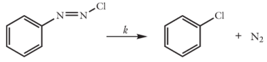
In the Model Builder window, under Component 1 (comp1) > Reaction Engineering (re) click 1: PhN2Cl => PhCl + N2.
2
In the Settings window for Reaction, locate the Rate Constants section.
3
Select the Use Arrhenius expressions checkbox.
4
In the Af text field, type exp(Aex).
5
In the Ef text field, type E.
Study 1
Parameter Estimation
1
In the Study toolbar, click  Optimization and choose Parameter Estimation.
2
In the Settings window for Parameter Estimation, locate the Estimated Parameters section.
3
Click  Add twice.
4
Use the Levenberg-Marquardt method to optimize this model.
5
Click to expand the Output section. Locate the Parameter Estimation Method section. From the Least-squares time/parameter list method list, choose Use only least-squares data points.
Setting the Least-squares time/parameter method to Use only least-squares data points will make the time dependent solver use the times specified by the experiments.
6
In the Study toolbar, click  Compute.
The solver has now optimized the model to find the values for the kinetic parameters. The values for the optimized parameters, as well as the value for the objective function, are found in Objective Probe Table 1.
Results
Objective Probe Table 1
E is found to be 1.16e5 J/mol and Aex is evaluated to 37.0.
The default plots illustrate the solution with the optimized parameter values, compared to each experimental data set used during parameter estimation. Simplify the legends and add a y-axis label.
Parameter estimation 313 K
1
In the Model Builder window, expand the Results > Tables node, then click Results > Parameter estimation.
2
In the Settings window for 1D Plot Group, type Parameter estimation 313 K in the Label text field.
3
Locate the Data section. From the Parameter selection (T_iso) list, choose From list.
4
In the Parameter values (T_iso) list box, select 313.
5
Locate the Plot Settings section. In the x-axis label text field, type Time (s).
6
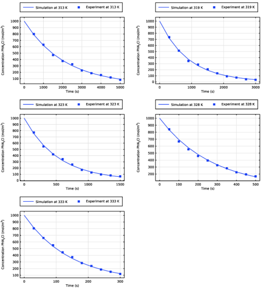
Select the y-axis label checkbox. In the associated text field, type Concentration PhN<sub>2</sub>Cl (mol/m<sup>3</sup>).
7
Locate the Legend section. From the Layout list, choose Outside graph axis area.
8
From the Position list, choose Top.
Simulation at 313 K
1
In the Model Builder window, expand the Parameter estimation 313 K node, then click Column 2 (model).
2
In the Settings window for Global, type Simulation at 313 K in the Label text field.
3
Click to expand the Legends section. Find the Include subsection. Select the Label checkbox.
4
Clear the Solution checkbox.
5
Clear the Expression checkbox.
Experiment at 313 K
1
In the Model Builder window, under Results > Parameter estimation 313 K click Column 2 (data).
2
In the Settings window for Global, type Experiment at 313 K in the Label text field.
3
Locate the Legends section. Find the Include subsection. Select the Label checkbox.
4
Clear the Solution checkbox.
5
Clear the Expression checkbox.
6
In the Parameter estimation 313 K toolbar, click  Plot.
Repeat the above steps for each default Parameter estimation plot.
Optionally, delete the generated default plot that was not used.
Concentration (re)
In the Model Builder window, under Results right-click Concentration (re) and choose Delete.