PDF

Chemical Vapor Deposition of Titanium Nitride on Machining Tool Inserts
Introduction
Chemical vapor deposition (CVD) is a process used to grow thin films on substrates. In this CVD example, metal inserts for machining tools are coated with titanium nitride (TiN). The titanium nitride layer improves the wear resistance of the metal inserts by increasing the hardness, reducing friction, and reducing oxidation. Additionally, due to its golden appearance, the coating process is also performed for aesthetic purposes.The CVD reactor in this example operates at low pressures and high temperatures. These operating conditions ensure high diffusion, which is needed for efficient mass transfer onto the substrate surfaces and for homogeneous deposition thicknesses (Ref. 1).
Model Definition
This model describes the coupled reaction kinetics, fluid flow, and mass transfer in the CVD reactor. The temperature is assumed to be held constant at 1100 K.
Model Geometry
The CVD reactor used in this coating process is made up of vertically stacked trays where each tray contains the metal inserts to be coated. Figure 1 illustrates one of these reactor trays where gas is fed from the center, reacts on the metal insert surfaces, and exits through the outer reactor wall.
Figure 1: Chemical vapor deposition reactor tray design used in this example.
Figure 2 shows the modeled domain which consists of a sixth of the full reactor tray shown in Figure 1 above. This simplification is made due to the symmetry of the reactor in order to reduce the computational time.
Figure 2: Model geometry including the domain and boundary labels. The labeled inserts (1 through 4) refer to the inserts that are studied in the Results and Discussion section.
Chemistry
The gas phase titanium chloride (TiCl4) reacts with nitrogen (N2) to form solid phase titanium nitrate (TiN) on the surface of the metal insert based on the following reaction:
(1)
The deposition rate (mol/(m2·s)) of TiN on the metal substrates is defined according to Popovska and others as follows (Ref. 1):
(2)
where pi is the nondimensional partial pressure of species i and k is the partially nondimensional rate constant (mol/(m2·s)) with reference pressure 1 Pa. The rate constant is described by the Arrhenius expression as follows:
(3)
where A is the partially nondimensional Arrhenius constant, 6.51 × 1016 mol/(m2·s) with reference pressure 1 Pa, and E is the activation energy, 7 × 103 J/mol (Ref. 1).
Fluid Flow
The fluid flow of the gas phase is described by the Navier–Stokes equations and is modeled assuming weakly compressible, laminar flow. The inlet of the gas has a normal mass flow rate boundary condition and the outlet of the gas has a pressure boundary condition where no backflow is enforced. Periodic flow boundary conditions are applied on the sides of the modeled geometry and there is no pressure drop across these boundaries.
Mass transfer
As seen in the chemical reaction (Equation 1), there are 5 species involved in the heterogeneous chemical reaction for the deposition process, four of which are gaseous species (TiCl4, N2, H2, and HCl) and one of which is a surface species (TiN).
The Transport of Concentrated Species interface is used to describe the mass transfer in the gas phase and is defined on all domains. This interface is used because there is no clear solvent choice, given the comparable amounts of the involved species, and because the gas density varies due to material removal during the adsorption reaction. The mass flux in the system consists of convective and diffusive flux. The diffusive flux is described with the mixture-averaged diffusion model. The gas inflow boundary condition is defined from a mole fraction. The surface reaction is modeled with a general inward flux boundary condition which is defined on the surface of the metal inserts as follows:
(4)
where ji is the mass flux (kg/(m2·s)), Mi is the molar mass (kg/mol), and Ri is the surface reaction rate (mol/(m2·s)) based on Equation 2 for species i (i = TiCl4, N2, H2, HCl). In an analogous manner to the fluid flow description, periodic condition boundaries are applied to the sides of the domain for mass transfer.
The Surface Reactions interface is used to describe the mass transfer in the adsorbed phase and is defined only on the surface of the metal inserts. The reaction rate for the surface species, TiN, is defined from Equation 2 (mol/(m2·s)). This interface is only enabled in the time-second study to solve for the time evolution of the deposition thickness.
computation
Two studies are computed in order to better understand how the mass flow rate affects the deposition rates, and how the position of tools within the tray affects deposition thickness:
1
2
Results and Discussion
Figure 3 below shows the deposition rate of TiN on the metal insert surfaces. The deposition rate on the surface of the metal inserts is the highest near the gas inlet and decreases over the distance where the reactants are consumed.
Figure 3: TiN deposition rate (m/s) on the metal insert surface and gas velocity field (m/s) streamlines for the mass flow rate base case (mfac = 1).
Figure 4 and Figure 5 show the deposition rate on four inserts and the variation between the homogeneity of the deposition rate. In both figures, the x-axis (mfac) refers to a factor of the base case inlet flow rate, 3.3 × 106 kg/s. The inserts 1 through 4 that are studied are indicated on the model domain geometry shown in Figure 2.
Figure 4: Average deposition rates for inserts 1 through 4 (m/h) and deposition rate homogeneity factor as a function of the inlet flow rate. The x-axis ‘mfac’ represents a factor of the base-case inlet flow rate, 3.3·10-6 kg/s.
Figure 4 shows that the metal insert located closest to the gas inlet (insert 1) has the highest deposition rate, whereas the metal insert located furthest from the gas inlet (insert 4) has the lowest deposition rate. This trend is due to the higher TiCl4 concentrations near the feed. Figure 4 also shows that higher total inlet mass flow rates result in higher depositions rate and also more uniform deposition rates between the metal insert locations in the tray.
Figure 5 shows another approach to comparing the homogeneity of the deposition by comparing the variation in the deposition rate.
Figure 5: Variation between the deposition rates for inserts 1 through 4.
Figure 5 clearly shows that, as the mass flow rate increases, there is less variation in the deposition rates across the insert surfaces.
Based on the trends shown in Figure 4 and Figure 5, a mass flow rate factor of 1, corresponding to an inlet flow rate of 3.3 × 106 kg/s, represents a good compromise between uniform deposition rates and efficient use of the injected gas feed. Therefore, this value is used in the second time-dependent study.
Figure 6 shows the deposition layer thickness for the metal inserts and the relative difference between insert 1 and insert 4 for the rotating insert section study.
Figure 6: Deposition layer thickness for inserts 1 through 4 (m) and the relative difference in thickness between insert 1 and insert 4 over time.
Figure 6 shows that the deposition layer thickness is rather uniform between the four inserts studied over time. Initially, the relative deposition thickness difference between insert 1 and insert 4 is approximately 1.6%. This value decreases in an oscillatory manner due to the rotation of the metal inserts until the relative difference is nearly negligible after 90 s. These results shows that the rotation results in a more uniform TiN coating thickness across all of the metal tools, compared to what is expected from the nonrotating (stationary) case.
Figure 7: TiN surface concentration (mol/m2) with contour plots showing the deposition thickness (m), the gas velocity (m/s) with arrows for the velocity field, and results at 90 s.
Figure 7 shows how the surface concentration of TiN on the metal inserts decreases toward the center of the subdomain containing the metal inserts due to the decrease in TiCl4 in the gas phase as the reaction progresses.
Reference
1. N. Popovska, S. Poscher, P. Tichy, G. Emig, and H. Ryssel, “Kinetics of Chemical Vapor Deposition of Titanium Nitride,” Electrochemical Society Proceedings, vol. 97, no. 25, pp. 592–596, 1997.
Application Library path: Chemical_Reaction_Engineering_Module/Reactors_with_Mass_Transfer/TiN_cvd_reactor
Modeling Instructions
From the File menu, choose New.
New
In the New window, click  Model Wizard.
Model Wizard
1
In the Model Wizard window, click  3D.
2
In the Select Physics tree, select Chemical Species Transport > Chemistry (chem).
3
Click Add.
4
In the Select Physics tree, select Chemical Species Transport > Transport of Concentrated Species (tcs).
5
Click Add.
6
In the Number of species text field, type 4.
7
In the Mass fractions (1) table, enter the following settings:
8
In the Select Physics tree, select Chemical Species Transport > Surface Reactions (sr).
9
Click Add.
10
In the Surface (adsorbed) species concentrations (mol/m²) table, enter the following settings:
11
In the Select Physics tree, select Fluid Flow > Single-Phase Flow > Laminar Flow (spf).
12
Click Add.
13
Click  Study.
14
In the Select Study tree, select General Studies > Stationary.
15
Global Definitions
Geometry Parameters
1
In the Model Builder window, under Global Definitions click Parameters 1.
2
In the Settings window for Parameters, type Geometry Parameters in the Label text field.
3
Locate the Parameters section. Click  Load from File.
4
Process Parameters
1
In the Home toolbar, click  Parameters and choose Add > Parameters.
2
In the Settings window for Parameters, type Process Parameters in the Label text field.
3
Locate the Parameters section. Click  Load from File.
4
Physical Parameters
1
In the Home toolbar, click  Parameters and choose Add > Parameters.
2
In the Settings window for Parameters, type Physical Parameters in the Label text field.
3
Locate the Parameters section. Click  Load from File.
4
Geometry 1
Work Plane 1 (wp1)
1
In the Geometry toolbar, click  Work Plane.
2
In the Settings window for Work Plane, locate the Plane Definition section.
3
In the z-coordinate text field, type -H/2.
4
Locate the Unite Objects section. Clear the Unite objects checkbox.
Work Plane 1 (wp1) > Plane Geometry
In the Model Builder window, click Plane Geometry.
Work Plane 1 (wp1) > Circle 1 (c1)
1
In the Work Plane toolbar, click  Circle.
2
In the Settings window for Circle, locate the Size and Shape section.
3
In the Radius text field, type rReactorIn.
4
In the Sector angle text field, type 360/sectors.
5
Locate the Rotation Angle section. In the Rotation text field, type 90-360/sectors/2.
Work Plane 1 (wp1) > Circle 2 (c2)
1
Right-click Component 1 (comp1) > Geometry 1 > Work Plane 1 (wp1) > Plane Geometry > Circle 1 (c1) and choose Duplicate.
2
In the Settings window for Circle, locate the Size and Shape section.
3
In the Radius text field, type rReactorOut.
Work Plane 1 (wp1) > Difference 1 (dif1)
1
In the Work Plane toolbar, click  Booleans and Partitions and choose Difference.
2
3
In the Settings window for Difference, locate the Difference section.
4
Click to select the  Activate Selection toggle button for Objects to subtract.
5
Work Plane 1 (wp1) > Circle 3 (c3)
1
In the Work Plane toolbar, click  Circle.
2
In the Settings window for Circle, locate the Size and Shape section.
3
In the Radius text field, type rRotating.
4
Locate the Position section. In the yw text field, type rRotatingCenter.
Work Plane 1 (wp1) > Difference 2 (dif2)
1
In the Work Plane toolbar, click  Booleans and Partitions and choose Difference.
2
3
In the Settings window for Difference, locate the Difference section.
4
Click to select the  Activate Selection toggle button for Objects to subtract.
5
6
Select the Keep objects to subtract checkbox.
7
In the Work Plane toolbar, click  Build All.
Extrude 1 (ext1)
1
In the Model Builder window, right-click Geometry 1 and choose Extrude.
2
In the Settings window for Extrude, locate the General section.
3
From the Extrude from list, choose Faces.
4
On the object wp1.dif2, select Boundary 1 only.
5
On the object wp1.c3, select Boundary 1 only.
6
Locate the Distances section. In the table, enter the following settings:
Cylinder 1 (cyl1)
1
In the Geometry toolbar, click  Cylinder.
2
In the Settings window for Cylinder, locate the Size and Shape section.
3
In the Radius text field, type rInjector.
4
In the Height text field, type 5*rInjector.
5
Locate the Position section. In the y text field, type 0.6*rReactorIn.
6
Locate the Axis section. From the Axis type list, choose y-axis.
7
Locate the Selections of Resulting Entities section. Select the Resulting objects selection checkbox.
Rotate 1 (rot1)
1
In the Geometry toolbar, click  Transforms and choose Rotate.
2
3
In the Settings window for Rotate, locate the Rotation section.
4
In the Angle text field, type -20.
5
Locate the Point on Axis of Rotation section. In the y text field, type rReactorIn.
Work Plane 2 (wp2)
1
In the Geometry toolbar, click  Work Plane.
2
In the Settings window for Work Plane, locate the Plane Definition section.
3
From the Plane list, choose xz-plane.
4
In the y-coordinate text field, type rReactorOut*0.985.
Work Plane 2 (wp2) > Plane Geometry
In the Model Builder window, click Plane Geometry.
Work Plane 2 (wp2) > Rectangle 1 (r1)
1
In the Work Plane toolbar, click  Rectangle.
2
In the Settings window for Rectangle, locate the Size and Shape section.
3
In the Width text field, type Wextractor.
4
In the Height text field, type Hextractor.
5
Locate the Position section. From the Base list, choose Center.
Work Plane 2 (wp2) > Fillet 1 (fil1)
1
In the Work Plane toolbar, click  Fillet.
2
Click the  Zoom Extents button in the Graphics toolbar.
3
On the object r1, select Points 1–4 only.
4
In the Settings window for Fillet, locate the Radius section.
5
In the Radius text field, type Hextractor*0.5.
Extrude 2 (ext2)
1
In the Model Builder window, right-click Geometry 1 and choose Extrude.
2
In the Settings window for Extrude, locate the Distances section.
3
4
Click to expand the Scales section. In the table, enter the following settings:
Difference 1 (dif1)
1
In the Geometry toolbar, click  Booleans and Partitions and choose Difference.
2
3
In the Settings window for Difference, locate the Difference section.
4
Click to select the  Activate Selection toggle button for Objects to subtract.
5
Select the objects ext1(1) and ext1(2) only.
6
Select the Keep objects to subtract checkbox.
7
Clear the Keep interior boundaries checkbox.
Union 1 (uni1)
1
In the Geometry toolbar, click  Booleans and Partitions and choose Union.
2
Select the objects dif1, ext1(1), and rot1 only.
Work Plane 3 (wp3)
1
In the Geometry toolbar, click  Work Plane.
2
In the Settings window for Work Plane, locate the Plane Definition section.
3
In the z-coordinate text field, type -H/2+Hinsert.
Work Plane 3 (wp3) > Plane Geometry
In the Model Builder window, click Plane Geometry.
Work Plane 3 (wp3) > Polygon 1 (pol1)
1
In the Work Plane toolbar, click  Polygon.
2
In the Settings window for Polygon, locate the Coordinates section.
3
Work Plane 3 (wp3) > Circle 1 (c1)
1
In the Work Plane toolbar, click  Circle.
2
In the Settings window for Circle, locate the Size and Shape section.
3
In the Radius text field, type Linsert/7.
4
Locate the Position section. In the yw text field, type Linsert*(1-cos(30[deg])*0.5).
Work Plane 3 (wp3) > Difference 1 (dif1)
1
In the Work Plane toolbar, click  Booleans and Partitions and choose Difference.
2
3
In the Settings window for Difference, locate the Difference section.
4
Click to select the  Activate Selection toggle button for Objects to subtract.
5
Work Plane 3 (wp3) > Fillet 1 (fil1)
1
In the Work Plane toolbar, click  Fillet.
2
In the Settings window for Fillet, locate the Points section.
3
Click to select the  Activate Selection toggle button for Vertices to fillet.
4
On the object dif1, select Points 1, 3, and 7 only.
5
Locate the Radius section. In the Radius text field, type 1.0[mm].
Work Plane 3 (wp3) > Move 1 (mov1)
1
In the Work Plane toolbar, click  Transforms and choose Move.
2
3
In the Settings window for Move, locate the Displacement section.
4
In the yw text field, type rRotatingCenter+rRotating*0.49.
Work Plane 3 (wp3) > Rotate 1 (rot1)
1
In the Work Plane toolbar, click  Transforms and choose Rotate.
2
3
In the Settings window for Rotate, locate the Input section.
4
Select the Keep input objects checkbox.
5
Locate the Rotation section. In the Angle text field, type 36.
6
Locate the Center of Rotation section. In the yw text field, type rRotatingCenter.
Work Plane 3 (wp3) > Rotate 2 (rot2)
1
In the Work Plane toolbar, click  Transforms and choose Rotate.
2
Click in the Graphics window and then press Ctrl+A to select both objects.
3
In the Settings window for Rotate, locate the Input section.
4
Select the Keep input objects checkbox.
5
Locate the Rotation section. In the Angle text field, type 72.
6
Locate the Center of Rotation section. In the yw text field, type rRotatingCenter.
Work Plane 3 (wp3) > Rotate 3 (rot3)
1
In the Work Plane toolbar, click  Transforms and choose Rotate.
2
Click in the Graphics window and then press Ctrl+A to select all objects.
3
In the Settings window for Rotate, locate the Input section.
4
Select the Keep input objects checkbox.
5
Locate the Rotation section. In the Angle text field, type 144.
6
Locate the Center of Rotation section. In the yw text field, type rRotatingCenter.
Work Plane 3 (wp3) > Copy 1 (copy1)
1
In the Work Plane toolbar, click  Transforms and choose Copy.
2
3
In the Settings window for Copy, locate the Displacement section.
4
In the yw text field, type -Linsert*1.00.
Work Plane 3 (wp3) > Rotate 4 (rot4)
1
In the Work Plane toolbar, click  Transforms and choose Rotate.
2
3
In the Settings window for Rotate, locate the Rotation section.
4
In the Angle text field, type 15.
5
Locate the Center of Rotation section. In the yw text field, type rRotatingCenter.
Work Plane 3 (wp3) > Rotate 5 (rot5)
1
In the Work Plane toolbar, click  Transforms and choose Rotate.
2
3
In the Settings window for Rotate, locate the Input section.
4
Select the Keep input objects checkbox.
5
Locate the Rotation section. In the Angle text field, type 90.
6
Locate the Center of Rotation section. In the yw text field, type rRotatingCenter.
Work Plane 3 (wp3) > Rotate 6 (rot6)
1
In the Work Plane toolbar, click  Transforms and choose Rotate.
2
Select the objects rot4 and rot5 only.
3
In the Settings window for Rotate, locate the Input section.
4
Select the Keep input objects checkbox.
5
Locate the Rotation section. In the Angle text field, type 180.
6
Locate the Center of Rotation section. In the yw text field, type rRotatingCenter.
Work Plane 3 (wp3) > Rotate 7 (rot7)
1
In the Work Plane toolbar, click  Transforms and choose Rotate.
2
Select the objects mov1, rot1, rot2(1), rot2(2), rot3(1), rot3(2), rot3(3), and rot3(4) only.
3
In the Settings window for Rotate, locate the Input section.
4
Select the Keep input objects checkbox.
5
Locate the Rotation section. In the Angle text field, type 72+36.
6
Locate the Center of Rotation section. In the yw text field, type rRotatingCenter.
Extrude 3 (ext3)
1
In the Model Builder window, right-click Geometry 1 and choose Extrude.
2
In the Settings window for Extrude, locate the Distances section.
3
4
Locate the Selections of Resulting Entities section. Select the Resulting objects selection checkbox.
5
From the Show in physics list, choose All levels.
Difference 2 (dif2)
1
In the Geometry toolbar, click  Booleans and Partitions and choose Difference.
2
Select the object ext1(2) only.
3
In the Settings window for Difference, locate the Difference section.
4
Click to select the  Activate Selection toggle button for Objects to subtract.
5
Click the  Paste Selection button for Objects to subtract.
6
In the Paste Selection dialog, type ext3 in the Selection text field.
7
Form Assembly
1
In the Model Builder window, under Component 1 (comp1) > Geometry 1 click Form Union (fin).
2
In the Settings window for Form Union/Assembly, type Form Assembly in the Label text field.
3
Locate the Form Union/Assembly section. From the Action list, choose Form an assembly.
Ignore Faces 1 (igf1)
1
In the Geometry toolbar, click  Virtual Operations and choose Ignore Faces.
2
On the object fin, select Boundary 9 only.
Cumulative Selections
In the Geometry toolbar, click  Selections and choose Cumulative Selections.
Inserts
1
Right-click Cumulative Selections and choose Cumulative Selection.
2
In the Settings window for Selection, type Inserts in the Label text field.
Injector
1
In the Model Builder window, right-click Cumulative Selections and choose Cumulative Selection.
2
In the Settings window for Selection, type Injector in the Label text field.
Cylinder 1 (cyl1)
1
In the Model Builder window, under Component 1 (comp1) > Geometry 1 click Cylinder 1 (cyl1).
2
In the Settings window for Cylinder, locate the Selections of Resulting Entities section.
3
Find the Cumulative selection subsection. From the Contribute to list, choose Injector.
Extrude 3 (ext3)
1
In the Model Builder window, click Extrude 3 (ext3).
2
In the Settings window for Extrude, locate the Selections of Resulting Entities section.
3
Find the Cumulative selection subsection. From the Contribute to list, choose Inserts.
4
In the Geometry toolbar, click  Build All.
Definitions
Variables 1
1
In the Model Builder window, expand the Component 1 (comp1) > Definitions node.
2
Right-click Definitions and choose Variables.
3
In the Settings window for Variables, locate the Variables section.
4
Click  Load from File.
5
Insert Boundary Variables
1
Right-click Definitions and choose Variables.
2
In the Settings window for Variables, type Insert Boundary Variables in the Label text field.
3
Locate the Geometric Entity Selection section. From the Geometric entity level list, choose Boundary.
4
From the Selection list, choose Inserts.
5
Locate the Variables section. Click  Load from File.
6
Step 1 (step1)
1
In the Definitions toolbar, click  More Functions and choose Step.
2
In the Settings window for Step, click to expand the Smoothing section.
3
In the Size of transition zone text field, type t_rot.
Inlet
1
In the Definitions toolbar, click  Explicit.
2
In the Settings window for Explicit, type Inlet in the Label text field.
3
Locate the Input Entities section. From the Geometric entity level list, choose Boundary.
4
Outlet
1
In the Definitions toolbar, click  Explicit.
2
In the Settings window for Explicit, type Outlet in the Label text field.
3
Locate the Input Entities section. From the Geometric entity level list, choose Boundary.
4
Rotating Domain
1
In the Definitions toolbar, click  Explicit.
2
In the Settings window for Explicit, type Rotating Domain in the Label text field.
3
Inserts Vertical Bnds
1
In the Definitions toolbar, click  Cylinder.
2
In the Settings window for Cylinder, type Inserts Vertical Bnds in the Label text field.
3
Locate the Geometric Entity Level section. From the Level list, choose Boundary.
4
Locate the Size and Shape section. In the Outer radius text field, type 0.99*rRotating.
5
In the Top distance text field, type 0.25*Hinsert.
6
In the Bottom distance text field, type -0.25*Hinsert.
7
Locate the Position section. In the y text field, type rRotatingCenter.
Insert Horizontal Edges
1
In the Definitions toolbar, click  Adjacent.
2
In the Settings window for Adjacent, type Insert Horizontal Edges in the Label text field.
3
Locate the Input Entities section. From the Geometric entity level list, choose Boundary.
4
Under Input selections, click  Add.
5
In the Add dialog, select Inserts Vertical Bnds in the Input selections list.
6
7
In the Settings window for Adjacent, locate the Output Entities section.
8
From the Geometric entity level list, choose Adjacent edges.
Insert Vertical Edges
1
In the Definitions toolbar, click  Adjacent.
2
In the Settings window for Adjacent, type Insert Vertical Edges in the Label text field.
3
Locate the Input Entities section. From the Geometric entity level list, choose Boundary.
4
Under Input selections, click  Add.
5
In the Add dialog, select Inserts Vertical Bnds in the Input selections list.
6
7
In the Settings window for Adjacent, locate the Output Entities section.
8
From the Geometric entity level list, choose Adjacent edges.
9
From the Exterior edges list, choose None.
10
Select the Interior edges checkbox.
Insert Top Bnds
1
In the Definitions toolbar, click  Cylinder.
2
In the Settings window for Cylinder, type Insert Top Bnds in the Label text field.
3
Locate the Geometric Entity Level section. From the Level list, choose Boundary.
4
Locate the Size and Shape section. In the Outer radius text field, type 0.99*rRotating.
5
In the Top distance text field, type Hinsert.
6
In the Bottom distance text field, type 0[mm].
7
Locate the Position section. In the y text field, type rRotatingCenter.
8
Locate the Output Entities section. From the Include entity if list, choose Entity inside cylinder.
Insert Bottom Bnds
1
In the Definitions toolbar, click  Cylinder.
2
In the Settings window for Cylinder, type Insert Bottom Bnds in the Label text field.
3
Locate the Geometric Entity Level section. From the Level list, choose Boundary.
4
Locate the Size and Shape section. In the Outer radius text field, type 0.036.
5
In the Top distance text field, type 0[mm].
6
In the Bottom distance text field, type -4[mm].
7
Locate the Position section. In the y text field, type rRotatingCenter.
8
Locate the Output Entities section. From the Include entity if list, choose Entity inside cylinder.
Sliding Mesh, Source Bnds
1
In the Definitions toolbar, click  Explicit.
2
In the Settings window for Explicit, type Sliding Mesh, Source Bnds in the Label text field.
3
Locate the Input Entities section. From the Geometric entity level list, choose Boundary.
4
5
Click the  Zoom to Selection button in the Graphics toolbar.
Sliding Mesh Destination Bnds
1
In the Definitions toolbar, click  Explicit.
2
In the Settings window for Explicit, type Sliding Mesh Destination Bnds in the Label text field.
3
Locate the Input Entities section. From the Geometric entity level list, choose Boundary.
4
Insert 1
1
In the Definitions toolbar, click  Cylinder.
2
In the Settings window for Cylinder, type Insert 1 in the Label text field.
3
Locate the Geometric Entity Level section. From the Level list, choose Boundary.
4
Locate the Size and Shape section. In the Outer radius text field, type Linsert*0.6.
5
Locate the Position section. In the y text field, type rRotatingCenter-(3/4)*rRotating.
6
Locate the Output Entities section. From the Include entity if list, choose Entity inside cylinder.
Insert 2
1
In the Definitions toolbar, click  Cylinder.
2
In the Settings window for Cylinder, type Insert 2 in the Label text field.
3
Locate the Geometric Entity Level section. From the Level list, choose Boundary.
4
Locate the Size and Shape section. In the Outer radius text field, type Linsert*0.6.
5
Locate the Position section. In the x text field, type Linsert*0.15.
6
In the y text field, type rRotatingCenter-(1/4)*rRotating.
7
Locate the Output Entities section. From the Include entity if list, choose Entity inside cylinder.
Insert 3
1
In the Definitions toolbar, click  Cylinder.
2
In the Settings window for Cylinder, type Insert 3 in the Label text field.
3
Locate the Geometric Entity Level section. From the Level list, choose Boundary.
4
Locate the Size and Shape section. In the Outer radius text field, type Linsert*0.6.
5
Locate the Position section. In the x text field, type -Linsert*0.15.
6
In the y text field, type rRotatingCenter+(1/4)*rRotating.
7
Locate the Output Entities section. From the Include entity if list, choose Entity inside cylinder.
Insert 4
1
In the Definitions toolbar, click  Cylinder.
2
In the Settings window for Cylinder, type Insert 4 in the Label text field.
3
Locate the Geometric Entity Level section. From the Level list, choose Boundary.
4
Locate the Size and Shape section. In the Outer radius text field, type Linsert*0.6.
5
Locate the Position section. In the y text field, type rRotatingCenter+(3/4)*rRotating.
6
Locate the Output Entities section. From the Include entity if list, choose Entity inside cylinder.
7
Click the  Show More Options button in the Model Builder toolbar.
8
In the Show More Options dialog, select Physics > Advanced Physics Options in the tree.
9
In the tree, select the checkbox for the node Physics > Advanced Physics Options.
10
11
Click the  Zoom Extents button in the Graphics toolbar.
Component 1 (comp1)
Rotating Domain 1
1
In the Physics toolbar, click  Moving Mesh and choose Rotating Domain.
2
In the Settings window for Rotating Domain, locate the Domain Selection section.
3
From the Selection list, choose Rotating Domain.
4
Locate the Rotation section. From the Rotation type list, choose Specified rotational velocity.
5
From the Rotational velocity expression list, choose General revolutions per time.
6
In the f text field, type rpm*step1(t).
7
Locate the Axis section. Specify the rax vector as
Multiphysics
Reacting Flow 1 (nirf1)
1
In the Physics toolbar, click  Multiphysics Couplings and choose Domain > Reacting Flow.
2
In the Settings window for Reacting Flow, locate the Coupled Interfaces section.
3
From the Chemistry (optional) list, choose None.
Chemistry (chem)
Reaction 1
1
In the Physics toolbar, click  Domains and choose Reaction.
2
In the Settings window for Reaction, locate the Reaction Formula section.
3
In the Formula text field, type 2 TiCl4 + N2 + 4 H2 => 2 TiN(ads) + 8 HCl.
4
Click Apply.
5
Locate the Reaction Rate section. From the list, choose User defined.
6
In the rj text field, type kPop*pTiCl4^1.25*pH2^0.5*pN2^0.5.
7
Locate the Reaction Orders section. Find the Volumetric overall reaction order subsection. In the Forward text field, type 1.
8
In the Model Builder window, click Chemistry (chem).
9
In the Settings window for Chemistry, locate the Model Input section.
10
From the T list, choose User defined. In the associated text field, type Treac.
11
From the p list, choose User defined. In the associated text field, type pRef.
12
Locate the Mixture Properties section. From the Type list, choose Concentrated species.
13
Locate the Species Matching section. Find the Bulk species subsection. From the Species solved for list, choose Transport of Concentrated Species.
14
15
Find the Surface species subsection. From the Species solved for list, choose Surface Reactions.
16
Species: TiCl4
1
In the Model Builder window, click Species: TiCl4.
2
In the Settings window for Species, click to expand the Transport Expressions section.
3
In the σ text field, type LJpot_TiCl4.
4
In the ε/kb text field, type epsilon_k_TiCl4.
Species: N2
1
In the Model Builder window, click Species: N2.
2
In the Settings window for Species, locate the Transport Expressions section.
3
In the σ text field, type LJpot_N2.
4
In the ε/kb text field, type epsilon_k_N2.
Species: H2
1
In the Model Builder window, click Species: H2.
2
In the Settings window for Species, locate the Transport Expressions section.
3
In the σ text field, type LJpot_H2.
4
In the ε/kb text field, type epsilon_k_H2.
Species: HCl
1
In the Model Builder window, click Species: HCl.
2
In the Settings window for Species, locate the Transport Expressions section.
3
In the σ text field, type LJpot_HCl.
Transport of Concentrated Species (tcs)
In the Model Builder window, under Component 1 (comp1) click Transport of Concentrated Species (tcs).
Inflow 1
In the Physics toolbar, click  Boundaries and choose Inflow.
Outflow 1
In the Physics toolbar, click  Boundaries and choose Outflow.
Flux 1
In the Physics toolbar, click  Boundaries and choose Flux.
Periodic Condition 1
In the Physics toolbar, click  Boundaries and choose Periodic Condition.
Fluid 1
1
In the Model Builder window, click Fluid 1.
2
In the Settings window for Fluid, locate the Model Input section.
3
From the T list, choose User defined. In the associated text field, type Treac.
4
Locate the Density section. From the ρ list, choose Density (chem).
5
Locate the Diffusion section. In the table, enter the following settings:
Initial Values 1
1
In the Model Builder window, click Initial Values 1.
2
In the Settings window for Initial Values, locate the Initial Values section.
3
From the Mixture specification list, choose Mole fractions.
4
In the x0,wN2 text field, type xN2in.
5
In the x0,wTiCl4 text field, type xTiCl4in.
6
In the x0,wHCl text field, type 1e-6.
Inflow 1
1
In the Model Builder window, click Inflow 1.
2
In the Settings window for Inflow, locate the Boundary Selection section.
3
From the Selection list, choose Inlet.
4
Locate the Inflow section. From the Mixture specification list, choose Mole fractions.
5
In the x0,wN2 text field, type xN2in.
6
In the x0,wTiCl4 text field, type xTiCl4in.
7
In the x0,wHCl text field, type 1e-6.
Outflow 1
1
In the Model Builder window, click Outflow 1.
2
In the Settings window for Outflow, locate the Boundary Selection section.
3
From the Selection list, choose Outlet.
Flux 1
1
In the Model Builder window, click Flux 1.
2
In the Settings window for Flux, locate the Boundary Selection section.
3
From the Selection list, choose Inserts.
4
Locate the Mass Transfer to Other Phases section. Select the Account for Stefan velocity checkbox.
5
Locate the Inward Flux section. Select the Species wH2 checkbox.
6
In the j0,wH2 text field, type chem.Rwsurf_H2.
7
Select the Species wN2 checkbox.
8
In the j0,wN2 text field, type chem.Rwsurf_N2.
9
Select the Species wTiCl4 checkbox.
10
In the j0,wTiCl4 text field, type chem.Rwsurf_TiCl4.
11
Select the Species wHCl checkbox.
12
In the j0,wHCl text field, type chem.Rwsurf_HCl.
Periodic Condition 1
1
In the Model Builder window, click Periodic Condition 1.
2
Surface Reactions (sr)
1
In the Model Builder window, under Component 1 (comp1) click Surface Reactions (sr).
2
In the Settings window for Surface Reactions, locate the Boundary Selection section.
3
From the Selection list, choose Inserts.
Surface Properties 1
1
In the Model Builder window, under Component 1 (comp1) > Surface Reactions (sr) click Surface Properties 1.
2
In the Settings window for Surface Properties, click to expand the Species Conservation on Deforming Geometry section.
3
Locate the Surface Diffusion section. In the DcTiN text field, type 1e-7.
Reactions 1
1
In the Physics toolbar, click  Boundaries and choose Reactions.
2
In the Settings window for Reactions, locate the Boundary Selection section.
3
From the Selection list, choose Inserts.
4
Locate the Reaction Rate for Surface Species section. From the Rs,cTiN list, choose Surface reaction rate for surface species TiN_surf (chem).
Laminar Flow (spf)
In the Model Builder window, under Component 1 (comp1) click Laminar Flow (spf).
Inlet 1
In the Physics toolbar, click  Boundaries and choose Inlet.
Outlet 1
In the Physics toolbar, click  Boundaries and choose Outlet.
Periodic Flow Condition 1
1
In the Physics toolbar, click  Boundaries and choose Periodic Flow Condition.
2
In the Model Builder window, click Laminar Flow (spf).
3
In the Settings window for Laminar Flow, locate the Physical Model section.
4
From the Compressibility list, choose Weakly compressible flow.
5
In the pref text field, type pRef.
6
In the Tref text field, type Treac.
Fluid Properties 1
1
In the Model Builder window, click Fluid Properties 1.
2
In the Settings window for Fluid Properties, locate the Fluid Properties section.
3
From the μ list, choose Dynamic viscosity (chem).
Inlet 1
1
In the Model Builder window, click Inlet 1.
2
In the Settings window for Inlet, locate the Boundary Selection section.
3
From the Selection list, choose Inlet.
4
Locate the Boundary Condition section. From the list, choose Mass flow.
5
Clear the Apply condition on each disjoint selection separately checkbox.
6
Locate the Mass Flow section. In the m text field, type mFlowIn.
7
Click to expand the Applicable Pair Region section. From the Allowed region list, choose All regions.
Outlet 1
1
In the Model Builder window, click Outlet 1.
2
In the Settings window for Outlet, locate the Boundary Selection section.
3
From the Selection list, choose Outlet.
Periodic Flow Condition 1
1
In the Model Builder window, click Periodic Flow Condition 1.
2
Mesh 1
Size 1
In the Model Builder window, under Component 1 (comp1) right-click Mesh 1 and choose Size.
Size
1
In the Settings window for Size, locate the Element Size section.
2
From the Calibrate for list, choose Fluid dynamics.
3
From the Predefined list, choose Coarse.
Size 1
1
In the Model Builder window, click Size 1.
2
In the Settings window for Size, locate the Geometric Entity Selection section.
3
From the Geometric entity level list, choose Boundary.
4
5
Locate the Element Size section. From the Calibrate for list, choose Fluid dynamics.
6
From the Predefined list, choose Fine.
Free Triangular 1
1
In the Mesh toolbar, click  More Generators and choose Free Triangular.
2
In the Settings window for Free Triangular, locate the Boundary Selection section.
3
From the Selection list, choose Inlet.
Size 1
1
Right-click Free Triangular 1 and choose Size.
2
In the Settings window for Size, locate the Element Size section.
3
From the Calibrate for list, choose Fluid dynamics.
4
Click the Custom button.
5
Locate the Element Size Parameters section.
6
Select the Maximum element size checkbox. In the associated text field, type 0.0015.
7
Select the Minimum element size checkbox. In the associated text field, type 0.5E-3.
8
Select the Maximum element growth rate checkbox.
9
Select the Curvature factor checkbox. In the associated text field, type 0.5.
10
Select the Resolution of narrow regions checkbox. In the associated text field, type 0.8.
Free Triangular 2
1
In the Mesh toolbar, click  More Generators and choose Free Triangular.
2
In the Settings window for Free Triangular, locate the Boundary Selection section.
3
From the Selection list, choose Insert Top Bnds.
Size 1
1
Right-click Free Triangular 2 and choose Size.
2
In the Settings window for Size, locate the Element Size section.
3
From the Calibrate for list, choose Fluid dynamics.
4
Click the Custom button.
5
Locate the Element Size Parameters section.
6
Select the Maximum element size checkbox. In the associated text field, type 0.004.
7
Select the Minimum element size checkbox. In the associated text field, type 2.54E-4.
8
Select the Maximum element growth rate checkbox.
9
Select the Curvature factor checkbox. In the associated text field, type 0.5.
Size 2
1
In the Model Builder window, right-click Free Triangular 2 and choose Size.
2
In the Settings window for Size, locate the Geometric Entity Selection section.
3
From the Geometric entity level list, choose Edge.
4
From the Selection list, choose Insert Horizontal Edges.
5
Locate the Element Size section. Click the Custom button.
6
Locate the Element Size Parameters section.
7
Select the Maximum element size checkbox. In the associated text field, type 0.00085.
Boundary Layers 1
1
In the Mesh toolbar, click  Boundary Layers.
2
In the Settings window for Boundary Layers, locate the Geometric Entity Selection section.
3
From the Geometric entity level list, choose Boundary.
4
From the Selection list, choose Insert Top Bnds.
Boundary Layer Properties
1
In the Model Builder window, click Boundary Layer Properties.
2
In the Settings window for Boundary Layer Properties, locate the Edge Selection section.
3
From the Selection list, choose Insert Horizontal Edges.
4
Locate the Layers section. In the Number of layers text field, type 1.
5
From the Thickness specification list, choose First layer.
6
In the Thickness text field, type 3E-4.
Copy Face 1
1
In the Mesh toolbar, click  Copy and choose Copy Face.
2
In the Settings window for Copy Face, locate the Source Boundaries section.
3
From the Selection list, choose Insert Top Bnds.
4
Locate the Destination Boundaries section. From the Selection list, choose Insert Bottom Bnds.
Mapped 1
1
In the Mesh toolbar, click  More Generators and choose Mapped.
2
In the Settings window for Mapped, locate the Boundary Selection section.
3
From the Selection list, choose Inserts Vertical Bnds.
Distribution 1
1
Right-click Mapped 1 and choose Distribution.
2
In the Settings window for Distribution, locate the Edge Selection section.
3
From the Selection list, choose Insert Vertical Edges.
4
Locate the Distribution section. From the Distribution type list, choose Predefined.
5
In the Number of elements text field, type 9.
6
In the Element ratio text field, type 2.
7
Select the Symmetric distribution checkbox.
Swept 1
1
In the Mesh toolbar, click  Swept.
2
In the Settings window for Swept, locate the Domain Selection section.
3
From the Geometric entity level list, choose Domain.
4
From the Selection list, choose Injector.
Distribution 1
1
Right-click Swept 1 and choose Distribution.
2
In the Settings window for Distribution, locate the Domain Selection section.
3
From the Selection list, choose Injector.
4
Locate the Distribution section. From the Distribution type list, choose Predefined.
5
In the Number of elements text field, type 10.
6
Select the Symmetric distribution checkbox.
Convert 1
1
In the Mesh toolbar, click  Modify and choose Convert.
2
In the Settings window for Convert, locate the Geometric Entity Selection section.
3
From the Geometric entity level list, choose Boundary.
4
From the Selection list, choose Inserts Vertical Bnds.
Free Tetrahedral 1
1
In the Mesh toolbar, click  Free Tetrahedral.
2
In the Settings window for Free Tetrahedral, locate the Domain Selection section.
3
From the Geometric entity level list, choose Domain.
4
From the Selection list, choose Rotating Domain.
Size 1
1
Right-click Free Tetrahedral 1 and choose Size.
2
In the Settings window for Size, locate the Geometric Entity Selection section.
3
From the Geometric entity level list, choose Boundary.
4
From the Selection list, choose Sliding Mesh Destination Bnds.
5
Locate the Element Size section. Click the Custom button.
6
Locate the Element Size Parameters section.
7
Select the Maximum element size checkbox. In the associated text field, type 0.00175.
Copy 1
1
In the Mesh toolbar, click  Copy and choose Copy.
2
In the Settings window for Copy, locate the Source Entities section.
3
From the Selection list, choose Sliding Mesh Destination Bnds.
4
Locate the Destination Entities section. From the Selection list, choose Sliding Mesh, Source Bnds.
Free Triangular 3
1
In the Mesh toolbar, click  More Generators and choose Free Triangular.
2
Size 1
1
Right-click Free Triangular 3 and choose Size.
2
In the Settings window for Size, locate the Element Size section.
3
From the Calibrate for list, choose Fluid dynamics.
4
Click the Custom button.
5
Locate the Element Size Parameters section.
6
Select the Maximum element size checkbox. In the associated text field, type 0.0013.
7
Select the Minimum element size checkbox. In the associated text field, type 0.0013/2.
8
Select the Maximum element growth rate checkbox. In the associated text field, type 1.05.
Copy 2
1
In the Mesh toolbar, click  Copy and choose Copy.
2
3
In the Settings window for Copy, locate the Destination Entities section.
4
Click to select the  Activate Selection toggle button.
5
Free Tetrahedral 2
In the Mesh toolbar, click  Free Tetrahedral.
Boundary Layers 2
1
In the Mesh toolbar, click  Boundary Layers.
2
In the Settings window for Boundary Layers, locate the Geometric Entity Selection section.
3
From the Geometric entity level list, choose Domain.
4
From the Selection list, choose All domains.
5
Click to expand the Corner Settings section. From the Handling of sharp edges list, choose Trimming.
Boundary Layer Properties
1
In the Model Builder window, click Boundary Layer Properties.
2
In the Settings window for Boundary Layer Properties, locate the Boundary Selection section.
3
Click  Paste Selection.
4
In the Paste Selection dialog, type 2-4, 7-9, 11-14, 19, 20, 26, 27, 31-124, 126-129, 131-202 in the Selection text field.
5
6
In the Settings window for Boundary Layer Properties, locate the Layers section.
7
In the Number of layers text field, type 3.
8
In the Thickness adjustment factor text field, type 4.
9
In the Model Builder window, right-click Mesh 1 and choose Build All.
Results
Mesh 1
1
In the Model Builder window, expand the Results node.
2
Right-click Results > Datasets and choose Mesh.
Mesh plot
1
In the Results toolbar, click  3D Plot Group.
2
In the Settings window for 3D Plot Group, type Mesh plot in the Label text field.
3
Locate the Plot Settings section. Select the Propagate hiding to lower dimensions checkbox.
Mesh 1
1
Right-click Mesh plot and choose Mesh.
2
In the Settings window for Mesh, locate the Level section.
3
From the Level list, choose Volume.
4
Locate the Coloring and Style section. From the Element color list, choose Size.
5
From the Color table list, choose TrafficLight.
6
From the Color table transformation list, choose Reverse.
7
Click to expand the Element Filter section. Select the Enable filter checkbox.
8
In the Expression text field, type z<0.
9
Click the  Show Grid button in the Graphics toolbar.
10
In the Mesh plot toolbar, click  Plot.
11
Click the  Zoom Extents button in the Graphics toolbar.
Study 1 - Stationary Insert Sections
1
In the Model Builder window, click Study 1.
2
In the Settings window for Study, type Study 1 - Stationary Insert Sections in the Label text field.
3
Locate the Study Settings section. Select the Store complete solver history checkbox.
Solution 1 (sol1)
In the Study toolbar, click  Show Default Solver.
Step 1: Stationary
1
In the Model Builder window, under Study 1 - Stationary Insert Sections click Step 1: Stationary.
2
In the Settings window for Stationary, locate the Physics and Variables Selection section.
3
In the Solve for column of the table, under Component 1 (comp1), clear the checkbox for Surface Reactions (sr).
4
Click to expand the Study Extensions section. Select the Auxiliary sweep checkbox.
5
6
7
In the Study toolbar, click  Compute.
Results
Exterior Walls
1
In the Results toolbar, click  More Datasets and choose Surface.
2
In the Settings window for Surface, type Exterior Walls in the Label text field.
3
Locate the Selection section. Click  Clear Selection.
4
Click  Paste Selection.
5
In the Paste Selection dialog, type 33-44, 49, 50, 55-66, 73-77, 80-82, 85-89, 91-95, 97-106, 110-114, 120-124, 131, 134-137, 139-143, 145, 146, 150-158, 160-167, 174, 177-186, 191, 192, 197-202 in the Selection text field.
6
Exterior Walls 1
1
Right-click Exterior Walls and choose Duplicate.
2
In the Settings window for Surface, locate the Selection section.
3
Click  Clear Selection.
4
Click  Paste Selection.
5
In the Paste Selection dialog, type 2-4, 7-9, 11-14, 19, 20, 26, 27, 31-124, 126-129, 131-202 in the Selection text field.
6
Reactor Walls
1
Right-click Exterior Walls 1 and choose Duplicate.
2
In the Settings window for Surface, type Reactor Walls in the Label text field.
3
Locate the Selection section. Click  Clear Selection.
4
Click  Paste Selection.
5
In the Paste Selection dialog, type 2, 3, 7-9, 11, 13, 14, 19, 26, 31 in the Selection text field.
6
Study 1, Cut Plane, z = 0
1
In the Results toolbar, click  Cut Plane.
2
In the Settings window for Cut Plane, type Study 1, Cut Plane, z = 0 in the Label text field.
3
Locate the Plane Data section. From the Plane list, choose xy-planes.
4
Click the  Show More Options button in the Model Builder toolbar.
5
In the Show More Options dialog, select Results > Views in the tree.
6
7
View 3D 5
1
In the Model Builder window, under Results right-click Views and choose View 3D.
2
In the Settings window for View 3D, locate the View section.
3
Clear the Show grid checkbox.
View 3D 6
1
Right-click Views and choose View 3D.
2
In the Settings window for View 3D, locate the View section.
3
Clear the Show grid checkbox.
TiN Deposition Rate
1
In the Model Builder window, under Results click Concentration, H2, Streamline (tcs).
2
In the Settings window for 3D Plot Group, type TiN Deposition Rate in the Label text field.
3
Locate the Data section. From the Parameter value (mfac) list, choose 1.
4
Click to expand the Title section. From the Title type list, choose Manual.
5
In the Title text area, type Surface and contours: TiN layer growth rate (m/s) Streamline: Velocity field.
6
In the Parameter indicator text field, type Mass flow factor = eval(mfac).
7
Locate the Plot Settings section. Clear the Plot dataset edges checkbox.
8
Locate the Color Legend section. From the Position list, choose Right double.
Streamline 1
1
In the Model Builder window, expand the TiN Deposition Rate node, then click Streamline 1.
2
In the Settings window for Streamline, locate the Expression section.
3
In the x-component text field, type u.
4
In the y-component text field, type v.
5
In the z-component text field, type w.
6
Locate the Streamline Positioning section. From the Positioning list, choose Uniform density.
7
In the Density level text field, type 8.5.
8
From the Advanced parameters list, choose Manual.
9
In the Terminating distance factor text field, type 0.25.
10
Locate the Coloring and Style section. Find the Point style subsection. From the Arrow length list, choose Normalized.
Color Expression
1
In the Model Builder window, expand the Streamline 1 node, then click Color Expression.
2
In the Settings window for Color Expression, locate the Expression section.
3
In the Expression text field, type spf.U.
4
Click to expand the Title section. From the Title type list, choose None.
5
Locate the Coloring and Style section. From the Color table list, choose Rainbow.
Selection 1
1
In the Model Builder window, right-click Streamline 1 and choose Selection.
2
Surface 1
1
In the Model Builder window, right-click TiN Deposition Rate and choose Surface.
2
In the Settings window for Surface, locate the Expression section.
3
In the Expression text field, type TiNgrowth.
4
Locate the Coloring and Style section. From the Color table list, choose Metasepia.
5
From the Color table transformation list, choose Reverse.
6
Click to expand the Quality section. From the Evaluation settings list, choose Manual.
7
From the Smoothing list, choose Inside geometry domains.
Selection 1
1
Right-click Surface 1 and choose Selection.
2
In the Settings window for Selection, locate the Selection section.
3
From the Selection list, choose Inserts.
Surface: Walls
1
In the Model Builder window, right-click TiN Deposition Rate and choose Surface.
2
In the Settings window for Surface, type Surface: Walls in the Label text field.
3
Locate the Data section. From the Dataset list, choose Reactor Walls.
4
Locate the Expression section. In the Expression text field, type 1.
5
Locate the Coloring and Style section. From the Coloring list, choose Uniform.
6
From the Color list, choose Gray.
Contour 1
1
Right-click TiN Deposition Rate and choose Contour.
2
In the Settings window for Contour, locate the Expression section.
3
In the Expression text field, type TiNgrowth.
4
Locate the Coloring and Style section. From the Coloring list, choose Uniform.
5
From the Color list, choose Gray.
6
Clear the Color legend checkbox.
Selection 1
1
Right-click Contour 1 and choose Selection.
2
In the Settings window for Selection, locate the Selection section.
3
From the Selection list, choose Inserts.
4
In the TiN Deposition Rate toolbar, click  Plot.
Concentration, H2, Surface (tcs), Concentration, HCl, Streamline (tcs), Concentration, HCl, Surface (tcs), Concentration, N2, Streamline (tcs), Concentration, N2, Surface (tcs), Concentration, TiCl4, Streamline (tcs), Concentration, TiCl4, Surface (tcs)
1
In the Model Builder window, under Results, Ctrl-click to select Concentration, H2, Surface (tcs), Concentration, N2, Streamline (tcs), Concentration, N2, Surface (tcs), Concentration, TiCl4, Streamline (tcs), Concentration, TiCl4, Surface (tcs), Concentration, HCl, Streamline (tcs), and Concentration, HCl, Surface (tcs).
2
Velocity and TiCl4 Mole Fraction
1
In the Settings window for 3D Plot Group, type Velocity and TiCl4 Mole Fraction in the Label text field.
2
Locate the Data section. From the Parameter value (mfac) list, choose 1.
3
Locate the Title section. From the Title type list, choose Manual.
4
In the Title text area, type Arrow Surface: Velocity field Slice: Inlet normalized mole fraction of TiCl4.
5
In the Parameter indicator text field, type Mass flow factor = eval(mfac).
6
Locate the Plot Settings section. Clear the Plot dataset edges checkbox.
7
Locate the Color Legend section. Select the Show maximum and minimum values checkbox.
8
Select the Show units checkbox.
9
Click to expand the Number Format section. Select the Manual color legend settings checkbox.
10
In the Precision text field, type 4.
Multislice 1
1
In the Model Builder window, expand the Velocity and TiCl4 Mole Fraction node.
2
Right-click Multislice 1 and choose Delete.
Insert Walls
1
Right-click Velocity and TiCl4 Mole Fraction and choose Surface.
2
In the Settings window for Surface, type Insert Walls in the Label text field.
3
Locate the Expression section. In the Expression text field, type 1.
Selection 1
1
Right-click Insert Walls and choose Selection.
2
In the Settings window for Selection, locate the Selection section.
3
From the Selection list, choose Inserts.
Material Appearance 1
1
In the Model Builder window, right-click Insert Walls and choose Material Appearance.
2
In the Settings window for Material Appearance, locate the Appearance section.
3
From the Appearance list, choose Custom.
4
From the Material type list, choose Gold.
Reactor Walls
1
In the Model Builder window, right-click Velocity and TiCl4 Mole Fraction and choose Surface.
2
In the Settings window for Surface, type Reactor Walls in the Label text field.
3
Locate the Data section. From the Dataset list, choose Reactor Walls.
4
Locate the Expression section. In the Expression text field, type 1.
5
Locate the Coloring and Style section. From the Coloring list, choose Uniform.
6
From the Color list, choose Gray.
Velocity, z = 0
1
Right-click Velocity and TiCl4 Mole Fraction and choose Arrow Surface.
2
In the Settings window for Arrow Surface, type Velocity, z = 0 in the Label text field.
3
Locate the Data section. From the Dataset list, choose Study 1, Cut Plane, z = 0.
4
From the Solution parameters list, choose From parent.
5
Locate the Expression section. In the x-component text field, type u.
6
In the y-component text field, type v.
7
In the z-component text field, type w.
8
Locate the Arrow Positioning section. In the Number of arrows text field, type 300.
9
Locate the Coloring and Style section. From the Arrow length list, choose Logarithmic.
10
From the Color list, choose White.
tcs.x_wTiCl4/xTiCl4in
1
Right-click Velocity and TiCl4 Mole Fraction and choose Slice.
2
In the Settings window for Slice, type tcs.x_wTiCl4/xTiCl4in in the Label text field.
3
Locate the Expression section. In the Expression text field, type tcs.x_wTiCl4/xTiCl4in.
4
Locate the Plane Data section. From the Plane list, choose xy-planes.
5
In the Planes text field, type 1.
6
Locate the Coloring and Style section. From the Color table list, choose Lagoon.
Velocity and TiCl4 Concentration, Periodic Flow
1
Right-click Velocity and TiCl4 Mole Fraction and choose Duplicate.
2
In the Settings window for 3D Plot Group, type Velocity and TiCl4 Concentration, Periodic Flow in the Label text field.
3
Locate the Data section. From the Parameter value (mfac) list, choose 5.
4
Locate the Title section. In the Title text area, type Slice: Velocity magnitude (m/s) Slice: Mole fraction TiCl4 Arrow Surface: Velocity field.
5
Locate the Color Legend section. Clear the Show units checkbox.
6
Locate the Number Format section. Clear the Manual color legend settings checkbox.
Arrow Surface
1
In the Model Builder window, expand the Velocity and TiCl4 Concentration, Periodic Flow node, then click Velocity, z = 0.
2
In the Settings window for Arrow Surface, type Arrow Surface in the Label text field.
3
Locate the Data section. From the Dataset list, choose From parent.
4
Locate the Arrow Positioning section. In the Number of arrows text field, type 200.
5
Locate the Coloring and Style section. From the Arrow length list, choose Proportional.
6
From the Color list, choose Gray.
Selection 1
1
Right-click Arrow Surface and choose Selection.
2
Slice 1
1
In the Model Builder window, under Results > Velocity and TiCl4 Concentration, Periodic Flow click tcs.x_wTiCl4/xTiCl4in.
2
In the Settings window for Slice, type Slice 1 in the Label text field.
3
Locate the Expression section. In the Expression text field, type spf.U.
4
Locate the Plane Data section. From the Plane list, choose zx-planes.
5
From the Entry method list, choose Coordinates.
6
In the y-coordinates text field, type range(0.05,0.02,0.11).
7
Locate the Coloring and Style section. From the Color table list, choose Prism.
8
Click to expand the Quality section. From the Evaluation settings list, choose Manual.
9
From the Smoothing list, choose Inside geometry domains.
Selection 1
1
Right-click Slice 1 and choose Selection.
2
Slice 2
1
In the Model Builder window, right-click Velocity and TiCl4 Concentration, Periodic Flow and choose Slice.
2
In the Settings window for Slice, locate the Expression section.
3
In the Expression text field, type tcs.x_wTiCl4.
4
Locate the Plane Data section. From the Plane list, choose xy-planes.
5
In the Planes text field, type 1.
6
Locate the Coloring and Style section. From the Color table list, choose Viridis.
7
From the Color table transformation list, choose Reverse.
Partial Pressures
1
In the Model Builder window, under Results click Pressure (spf).
2
In the Settings window for 3D Plot Group, type Partial Pressures in the Label text field.
3
Locate the Data section. From the Parameter value (mfac) list, choose 1.
4
Locate the Title section. From the Title type list, choose Manual.
5
In the Title text area, type Partial Pressure.
6
In the Parameter indicator text field, type Mass flow factor = eval(mfac).
7
Locate the Plot Settings section. From the View list, choose View 3D 5.
8
Clear the Plot dataset edges checkbox.
9
Locate the Color Legend section. Select the Show maximum and minimum values checkbox.
10
Select the Show units checkbox.
11
From the Position list, choose Right double.
12
Locate the Number Format section. Select the Manual color legend settings checkbox.
13
In the Precision text field, type 4.
14
Click to expand the Plot Array section. From the Array type list, choose Square.
15
From the Order list, choose Column-major.
----> N2
1
Right-click Partial Pressures and choose Annotation.
2
In the Settings window for Annotation, type ----> N2 in the Label text field.
3
Locate the Annotation section. In the Text text field, type N2.
4
Locate the Position section. In the x text field, type -rReactorOut/2.
5
In the y text field, type rReactorOut/2.
6
Click to expand the Advanced section. Locate the Coloring and Style section. Clear the Show point checkbox.
7
From the Anchor point list, choose Center.
8
Right-click ----> N2 and choose Move Up.
Insert Walls
1
In the Model Builder window, under Results > Partial Pressures click Surface.
2
In the Settings window for Surface, type Insert Walls in the Label text field.
3
Locate the Expression section. In the Expression text field, type 1.
4
Locate the Coloring and Style section. Clear the Color legend checkbox.
5
Locate the Quality section. From the Smoothing list, choose Inside material domains.
6
Click to expand the Plot Array section. Select the Manual indexing checkbox.
Selection 1
1
In the Model Builder window, expand the Insert Walls node, then click Selection 1.
2
In the Settings window for Selection, locate the Selection section.
3
From the Selection list, choose Inserts.
Material Appearance 1
1
In the Model Builder window, right-click Insert Walls and choose Material Appearance.
2
In the Settings window for Material Appearance, locate the Appearance section.
3
From the Appearance list, choose Custom.
4
From the Material type list, choose Gold.
Reactor Walls
1
In the Model Builder window, right-click Partial Pressures and choose Surface.
2
In the Settings window for Surface, type Reactor Walls in the Label text field.
3
Locate the Data section. From the Dataset list, choose Reactor Walls.
4
Locate the Expression section. In the Expression text field, type 1.
5
Locate the Coloring and Style section. From the Coloring list, choose Uniform.
6
From the Color list, choose Gray.
7
Locate the Plot Array section. Select the Manual indexing checkbox.
pA_N2
1
Right-click Partial Pressures and choose Slice.
2
In the Settings window for Slice, type pA_N2 in the Label text field.
3
Locate the Expression section. In the Expression text field, type chem.pA_N2.
4
Locate the Plane Data section. From the Plane list, choose xy-planes.
5
In the Planes text field, type 1.
6
Locate the Coloring and Style section. From the Color table list, choose Metasepia.
7
Click to expand the Plot Array section. Select the Manual indexing checkbox.
----> TiCl4
1
Right-click Partial Pressures and choose Annotation.
2
In the Settings window for Annotation, type ----> TiCl4 in the Label text field.
3
Locate the Annotation section. In the Text text field, type TiCl4.
4
Locate the Position section. In the x text field, type -rReactorOut/2.
5
In the y text field, type rReactorOut/2.
6
Locate the Coloring and Style section. Clear the Show point checkbox.
7
From the Anchor point list, choose Center.
8
Click to expand the Plot Array section. Select the Manual indexing checkbox.
9
In the Row index text field, type -1.
Insert Walls 1
1
In the Model Builder window, right-click Insert Walls and choose Duplicate.
2
In the Settings window for Surface, locate the Plot Array section.
3
In the Row index text field, type -1.
Reactor Walls 1
1
In the Model Builder window, right-click Reactor Walls and choose Duplicate.
2
In the Settings window for Surface, locate the Plot Array section.
3
In the Row index text field, type -1.
pA_TiCl4
1
In the Model Builder window, right-click pA_N2 and choose Duplicate.
2
In the Settings window for Slice, type pA_TiCl4 in the Label text field.
3
Locate the Expression section. In the Expression text field, type chem.pA_TiCl4.
4
Locate the Coloring and Style section. From the Color table list, choose Lagoon.
5
Locate the Plot Array section. In the Row index text field, type -1.
----> H2
1
In the Model Builder window, right-click ----> TiCl4 and choose Duplicate.
2
In the Settings window for Annotation, type ----> H2 in the Label text field.
3
Locate the Annotation section. In the Text text field, type H2.
4
Locate the Plot Array section. In the Row index text field, type 0.
5
In the Column index text field, type 1.
Insert Walls 2
1
In the Model Builder window, right-click Insert Walls 1 and choose Duplicate.
2
In the Settings window for Surface, type Insert Walls 2 in the Label text field.
3
Locate the Plot Array section. In the Row index text field, type 0.
4
In the Column index text field, type 1.
Reactor Walls 2
1
In the Model Builder window, right-click Reactor Walls 1 and choose Duplicate.
2
In the Settings window for Surface, type Reactor Walls 2 in the Label text field.
3
Locate the Plot Array section. In the Row index text field, type 0.
4
In the Column index text field, type 1.
pA_H2
1
In the Model Builder window, right-click pA_TiCl4 and choose Duplicate.
2
In the Settings window for Slice, type pA_H2 in the Label text field.
3
Locate the Expression section. In the Expression text field, type chem.pA_H2.
4
Locate the Coloring and Style section. From the Color table list, choose Baptisia.
5
Locate the Plot Array section. In the Row index text field, type 0.
6
In the Column index text field, type 1.
----> HCl
1
In the Model Builder window, right-click ----> H2 and choose Duplicate.
2
In the Settings window for Annotation, type ----> HCl in the Label text field.
3
Locate the Annotation section. In the Text text field, type HCl.
4
Locate the Plot Array section. In the Row index text field, type -1.
Insert Walls 3
1
In the Model Builder window, right-click Insert Walls 2 and choose Duplicate.
2
In the Settings window for Surface, type Insert Walls 3 in the Label text field.
3
Locate the Plot Array section. In the Row index text field, type -1.
Reactor Walls 2.1
1
In the Model Builder window, right-click Reactor Walls 2 and choose Duplicate.
2
In the Settings window for Surface, locate the Plot Array section.
3
In the Row index text field, type -1.
pA_HCl
1
In the Model Builder window, right-click pA_H2 and choose Duplicate.
2
In the Settings window for Slice, type pA_HCl in the Label text field.
3
Locate the Expression section. In the Expression text field, type chem.pA_HCl.
4
Locate the Plot Array section. In the Row index text field, type -1.
Partial Pressures
1
In the Model Builder window, right-click Partial Pressures and choose Move Down.
2
In the Partial Pressures toolbar, click  Plot.
3
Click the  Zoom Extents button in the Graphics toolbar.
Average Deposition Rates
1
In the Results toolbar, click  Evaluation Group.
2
In the Settings window for Evaluation Group, type Average Deposition Rates in the Label text field.
3
Locate the Transformation section. From the Transformation type list, choose General.
4
Select the Keep child nodes checkbox.
Surface Average 1
1
Right-click Average Deposition Rates and choose Average > Surface Average.
2
In the Settings window for Surface Average, locate the Selection section.
3
From the Selection list, choose Insert 1.
4
Locate the Expressions section. In the table, enter the following settings:
Surface Average 2
1
Right-click Surface Average 1 and choose Duplicate.
2
In the Settings window for Surface Average, locate the Selection section.
3
From the Selection list, choose Insert 2.
4
Locate the Expressions section. In the table, enter the following settings:
Surface Average 3
1
Right-click Surface Average 2 and choose Duplicate.
2
In the Settings window for Surface Average, locate the Selection section.
3
From the Selection list, choose Insert 3.
4
Locate the Expressions section. In the table, enter the following settings:
Surface Average 4
1
Right-click Surface Average 3 and choose Duplicate.
2
In the Settings window for Surface Average, locate the Selection section.
3
From the Selection list, choose Insert 4.
4
Locate the Expressions section. In the table, enter the following settings:
Average Deposition Rates
1
In the Model Builder window, click Average Deposition Rates.
2
In the Settings window for Evaluation Group, locate the Transformation section.
3
In the Expression text field, type av1/av4.
4
In the Column header text field, type Insert1 / Insert4.
5
In the Average Deposition Rates toolbar, click  Evaluate.
Deposition Variation, Insert 1
1
In the Results toolbar, click  Evaluation Group.
2
In the Settings window for Evaluation Group, type Deposition Variation, Insert 1 in the Label text field.
3
Locate the Transformation section. From the Transformation type list, choose General.
4
Select the Keep child nodes checkbox.
Surface Maximum 1
1
Right-click Deposition Variation, Insert 1 and choose Maximum > Surface Maximum.
2
In the Settings window for Surface Maximum, locate the Selection section.
3
From the Selection list, choose Insert 1.
4
Locate the Expressions section. In the table, enter the following settings:
Surface Minimum 1
1
In the Model Builder window, right-click Deposition Variation, Insert 1 and choose Minimum > Surface Minimum.
2
In the Settings window for Surface Minimum, locate the Selection section.
3
From the Selection list, choose Insert 1.
4
Locate the Expressions section. In the table, enter the following settings:
Surface Average 1
1
Right-click Deposition Variation, Insert 1 and choose Average > Surface Average.
2
In the Settings window for Surface Average, locate the Selection section.
3
From the Selection list, choose Insert 1.
4
Locate the Expressions section. In the table, enter the following settings:
Deposition Variation, Insert 1
1
In the Model Builder window, click Deposition Variation, Insert 1.
2
In the Settings window for Evaluation Group, locate the Transformation section.
3
In the Expression text field, type (max1-min1)/av1.
4
In the Column header text field, type (Max-Min)/Average.
5
In the Deposition Variation, Insert 1 toolbar, click  Evaluate.
Deposition Variation, Insert 2
1
Right-click Deposition Variation, Insert 1 and choose Duplicate.
2
In the Model Builder window, click Deposition Variation, Insert 1.1.
3
In the Settings window for Evaluation Group, type Deposition Variation, Insert 2 in the Label text field.
Surface Maximum 1
1
In the Model Builder window, click Surface Maximum 1.
2
In the Settings window for Surface Maximum, locate the Selection section.
3
From the Selection list, choose Insert 2.
Surface Minimum 1
1
In the Model Builder window, click Surface Minimum 1.
2
In the Settings window for Surface Minimum, locate the Selection section.
3
From the Selection list, choose Insert 2.
Surface Average 1
1
In the Model Builder window, click Surface Average 1.
2
In the Settings window for Surface Average, locate the Selection section.
3
From the Selection list, choose Insert 2.
Deposition Variation, Insert 2
1
In the Model Builder window, click Deposition Variation, Insert 2.
2
In the Deposition Variation, Insert 2 toolbar, click  Evaluate.
Deposition Variation, Insert 3
1
Right-click Deposition Variation, Insert 2 and choose Duplicate.
2
In the Model Builder window, click Deposition Variation, Insert 2.1.
3
In the Settings window for Evaluation Group, type Deposition Variation, Insert 3 in the Label text field.
Surface Maximum 1
1
In the Model Builder window, click Surface Maximum 1.
2
In the Settings window for Surface Maximum, locate the Selection section.
3
From the Selection list, choose Insert 3.
Surface Minimum 1
1
In the Model Builder window, click Surface Minimum 1.
2
In the Settings window for Surface Minimum, locate the Selection section.
3
From the Selection list, choose Insert 3.
Surface Average 1
1
In the Model Builder window, click Surface Average 1.
2
In the Settings window for Surface Average, locate the Selection section.
3
From the Selection list, choose Insert 3.
Deposition Variation, Insert 3
1
In the Model Builder window, click Deposition Variation, Insert 3.
2
In the Deposition Variation, Insert 3 toolbar, click  Evaluate.
Deposition Variation, Insert 4
1
Right-click Deposition Variation, Insert 3 and choose Duplicate.
2
In the Model Builder window, click Deposition Variation, Insert 3.1.
3
In the Settings window for Evaluation Group, type Deposition Variation, Insert 4 in the Label text field.
Surface Maximum 1
1
In the Model Builder window, click Surface Maximum 1.
2
In the Settings window for Surface Maximum, locate the Selection section.
3
From the Selection list, choose Insert 4.
Surface Minimum 1
1
In the Model Builder window, click Surface Minimum 1.
2
In the Settings window for Surface Minimum, locate the Selection section.
3
From the Selection list, choose Insert 4.
Surface Average 1
1
In the Model Builder window, click Surface Average 1.
2
In the Settings window for Surface Average, locate the Selection section.
3
From the Selection list, choose Insert 4.
Deposition Variation, Insert 4
1
In the Model Builder window, click Deposition Variation, Insert 4.
2
In the Deposition Variation, Insert 4 toolbar, click  Evaluate.
Average Deposition Rate
1
In the Results toolbar, click  1D Plot Group.
2
In the Settings window for 1D Plot Group, type Average Deposition Rate in the Label text field.
3
Locate the Data section. From the Dataset list, choose None.
4
Locate the Plot Settings section.
5
Select the y-axis label checkbox. In the associated text field, type Deposition rate (um/h).
6
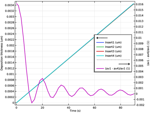
Select the Two y-axes checkbox.
Table Graph 1
1
Right-click Average Deposition Rate and choose Table Graph.
2
In the Settings window for Table Graph, locate the Data section.
3
From the Source list, choose Evaluation group.
4
From the Plot columns list, choose Manual.
5
In the Columns list, choose Insert1 (um/h), Insert2 (um/h), Insert3 (um/h), and Insert4 (um/h).
6
Locate the Coloring and Style section. From the Width list, choose 2.
7
Find the Line markers subsection. From the Marker list, choose Point.
8
Click to expand the Legends section. Select the Show legends checkbox.
Table Graph 2
1
In the Model Builder window, right-click Average Deposition Rate and choose Table Graph.
2
In the Settings window for Table Graph, locate the Data section.
3
From the Source list, choose Evaluation group.
4
From the Plot columns list, choose Manual.
5
In the Columns list box, select Insert1 / Insert4 (1).
6
Locate the y-Axis section. Select the Plot on secondary y-axis checkbox.
7
Locate the Coloring and Style section. From the Width list, choose 2.
8
Find the Line markers subsection. From the Marker list, choose Point.
9
Locate the Legends section. Select the Show legends checkbox.
Average Deposition Rate
1
In the Model Builder window, click Average Deposition Rate.
2
In the Average Deposition Rate toolbar, click  Plot.
3
In the Settings window for 1D Plot Group, locate the Axis section.
4
Select the Manual axis limits checkbox.
5
In the x minimum text field, type 0.14277.
6
In the x maximum text field, type 5.05723.
7
In the y minimum text field, type 0.12960.
8
In the y maximum text field, type 0.13998.
9
In the Secondary y minimum text field, type 0.95.
10
In the Secondary y maximum text field, type 1.05.
11
Locate the Legend section. From the Position list, choose Middle right.
12
In the Average Deposition Rate toolbar, click  Plot.
13
Click the  Zoom Extents button in the Graphics toolbar.
Max-Min Deposition Variation Over Inserts
1
In the Results toolbar, click  1D Plot Group.
2
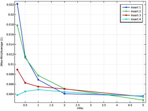
In the Settings window for 1D Plot Group, type Max-Min Deposition Variation Over Inserts in the Label text field.
3
Locate the Data section. From the Dataset list, choose None.
4
Click to expand the Title section. From the Title type list, choose Manual.
5
In the Title text area, type Deposition Variation Per Insert.
Table Graph 1
1
Right-click Max-Min Deposition Variation Over Inserts and choose Table Graph.
2
In the Settings window for Table Graph, locate the Data section.
3
From the Source list, choose Evaluation group.
4
From the Evaluation group list, choose Deposition Variation, Insert 1.
5
From the Plot columns list, choose Manual.
6
In the Columns list box, select (Max-Min)/Average (1).
7
Locate the Coloring and Style section. From the Width list, choose 2.
8
Find the Line markers subsection. From the Marker list, choose Point.
9
Locate the Legends section. Select the Show legends checkbox.
10
From the Legends list, choose Manual.
11
Table Graph 2
1
Right-click Table Graph 1 and choose Duplicate.
2
In the Settings window for Table Graph, locate the Data section.
3
From the Evaluation group list, choose Deposition Variation, Insert 2.
4
Locate the Legends section. In the table, enter the following settings:
Table Graph 3
1
Right-click Table Graph 2 and choose Duplicate.
2
In the Settings window for Table Graph, locate the Data section.
3
From the Evaluation group list, choose Deposition Variation, Insert 3.
4
Locate the Legends section. In the table, enter the following settings:
Table Graph 4
1
Right-click Table Graph 3 and choose Duplicate.
2
In the Settings window for Table Graph, locate the Data section.
3
From the Evaluation group list, choose Deposition Variation, Insert 4.
4
Locate the Legends section. In the table, enter the following settings:
5
In the Max-Min Deposition Variation Over Inserts toolbar, click  Plot.
Average Deposition Rate, Max-Min Deposition Variation Over Inserts, Partial Pressures, TiN Deposition Rate, Velocity and TiCl4 Concentration, Periodic Flow, Velocity and TiCl4 Mole Fraction
1
In the Model Builder window, under Results, Ctrl-click to select TiN Deposition Rate, Velocity and TiCl4 Mole Fraction, Velocity and TiCl4 Concentration, Periodic Flow, Partial Pressures, Average Deposition Rate, and Max-Min Deposition Variation Over Inserts.
2
Stationary Insert Sections
In the Settings window for Group, type Stationary Insert Sections in the Label text field.
Surface Reactions (sr)
Surface Properties 1
1
In the Model Builder window, under Component 1 (comp1) > Surface Reactions (sr) click Surface Properties 1.
2
In the Settings window for Surface Properties, locate the Species Conservation on Deforming Geometry section.
3
Clear the Compensate for boundary stretching checkbox.
Add Study
1
In the Study toolbar, click  Add Study to open the Add Study window.
2
Go to the Add Study window.
3
Find the Studies subsection. In the Select Study tree, select General Studies > Time Dependent.
4
Click the Add Study button in the window toolbar.
5
In the Study toolbar, click  Add Study to close the Add Study window.
Study 2 - Rotating Insert Sections
1
In the Settings window for Study, type Study 2 - Rotating Insert Sections in the Label text field.
2
Locate the Study Settings section. Clear the Generate default plots checkbox.
Step 1: Time Dependent
1
In the Model Builder window, under Study 2 - Rotating Insert Sections click Step 1: Time Dependent.
2
In the Settings window for Time Dependent, locate the Study Settings section.
3
In the Output times text field, type 0 6*t_rot.
4
Click to expand the Values of Dependent Variables section. Find the Initial values of variables solved for subsection. From the Settings list, choose User controlled.
5
From the Method list, choose Solution.
6
From the Study list, choose Study 1 - Stationary Insert Sections, Stationary.
7
From the Solution list, choose Solution 1 (sol1).
8
From the Parameter value (mfac) list, choose 1.
Solution 2 (sol2)
1
In the Study toolbar, click  Show Default Solver.
2
In the Model Builder window, expand the Solution 2 (sol2) node.
3
In the Model Builder window, under Study 2 - Rotating Insert Sections > Solver Configurations > Solution 2 (sol2) click Dependent Variables 1.
4
In the Settings window for Dependent Variables, locate the Residual Scaling section.
5
In the Threshold for updating residual scale text field, type 1.
6
In the Model Builder window, under Study 2 - Rotating Insert Sections > Solver Configurations > Solution 2 (sol2) > Dependent Variables 1 click Surface Concentration (comp1.cTiN).
7
In the Settings window for Field, locate the Scaling section.
8
From the Method list, choose Manual.
9
In the Scale text field, type 1e-4.
10
In the Model Builder window, under Study 2 - Rotating Insert Sections > Solver Configurations > Solution 2 (sol2) click Time-Dependent Solver 1.
11
In the Settings window for Time-Dependent Solver, locate the General section.
12
From the Times to store list, choose Steps taken by solver.
13
In the Store every Nth step text field, type 8.
14
Click to expand the Time Stepping section. Select the Initial step checkbox.
15
In the Study toolbar, click  Compute.
Results
Sector 3D 1
1
In the Results toolbar, click  More Datasets and choose Sector 3D.
2
In the Settings window for Sector 3D, locate the Data section.
3
From the Dataset list, choose Study 2 - Rotating Insert Sections/Solution 2 (sol2).
4
Locate the Symmetry section. In the Number of sectors text field, type 6.
5
From the Sectors to include list, choose Manual.
Study 2/Solution 2, Reactor Walls
1
In the Model Builder window, under Results > Datasets right-click Study 2 - Rotating Insert Sections/Solution 2 (sol2) and choose Duplicate.
2
In the Settings window for Solution, type Study 2/Solution 2, Reactor Walls in the Label text field.
Selection
1
In the Results toolbar, click  Attributes and choose Selection.
2
In the Settings window for Selection, locate the Geometric Entity Selection section.
3
From the Geometric entity level list, choose Boundary.
4
Click  Paste Selection.
5
In the Paste Selection dialog, type 2, 3, 7-9, 11-14, 19, 20, 26, 27, 31 in the Selection text field.
6
Sector 3D 2
1
In the Results toolbar, click  More Datasets and choose Sector 3D.
2
In the Settings window for Sector 3D, locate the Data section.
3
From the Dataset list, choose Study 2/Solution 2, Reactor Walls (sol2).
4
Locate the Symmetry section. In the Number of sectors text field, type 6.
5
From the Sectors to include list, choose Manual.
Sector 3D, Cut Plane, z = 0
1
In the Results toolbar, click  Cut Plane.
2
In the Settings window for Cut Plane, type Sector 3D, Cut Plane, z = 0 in the Label text field.
3
Locate the Data section. From the Dataset list, choose Sector 3D 1.
4
Locate the Plane Data section. From the Plane list, choose xy-planes.
Rotating Insert Sections
1
In the Model Builder window, right-click Stationary Insert Sections and choose Duplicate.
2
In the Model Builder window, click Stationary Insert Sections 1.
3
In the Settings window for Group, type Rotating Insert Sections in the Label text field.
Full Reactor: Flow and Deposited TiN
1
In the Model Builder window, under Results > Rotating Insert Sections click TiN Deposition Rate 1.
2
In the Settings window for 3D Plot Group, type Full Reactor: Flow and Deposited TiN in the Label text field.
3
Locate the Data section. From the Dataset list, choose Sector 3D 1.
4
From the Time (s) list, choose Last (90).
5
Locate the Title section. In the Title text area, type Velocity, Inlet Normalized TiCl4 Concentration, and Deposited TiN.
6
In the Parameter indicator text field, type Time = eval(t) s.
7
Locate the Plot Settings section. From the View list, choose View 3D 6.
8
Locate the Color Legend section. Select the Show maximum and minimum values checkbox.
9
Select the Show units checkbox.
10
Locate the Number Format section. Select the Manual color legend settings checkbox.
11
In the Precision text field, type 4.
Streamline 1
1
In the Model Builder window, expand the Full Reactor: Flow and Deposited TiN node.
2
Right-click Streamline 1 and choose Delete.
Insert Walls
1
In the Settings window for Surface, type Insert Walls in the Label text field.
2
Locate the Expression section. In the Expression text field, type 1.
3
Locate the Quality section. From the Smoothing list, choose Inside material domains.
Material Appearance 1
Right-click Insert Walls and choose Material Appearance.
Material Appearance 1
1
In the Model Builder window, expand the Results > Rotating Insert Sections > Full Reactor: Flow and Deposited TiN > Insert Walls node, then click Material Appearance 1.
2
In the Settings window for Material Appearance, locate the Appearance section.
3
From the Appearance list, choose Custom.
4
From the Material type list, choose Gold.
Reactor Walls
1
In the Model Builder window, under Results > Rotating Insert Sections > Full Reactor: Flow and Deposited TiN click Surface: Walls.
2
In the Settings window for Surface, type Reactor Walls in the Label text field.
3
Locate the Data section. From the Dataset list, choose Sector 3D 2.
4
From the Time (s) list, choose 0.
Contour 1
1
In the Model Builder window, click Contour 1.
2
In the Settings window for Contour, locate the Expression section.
3
In the Expression text field, type cTiN*chem.M_TiN_surf/rhoTiN.
4
Locate the Levels section. In the Total levels text field, type 10.
5
Locate the Coloring and Style section. From the Color list, choose White.
6
Select the Color legend checkbox.
Velocity, z = 0
1
In the Model Builder window, right-click Full Reactor: Flow and Deposited TiN and choose Arrow Surface.
2
In the Settings window for Arrow Surface, type Velocity, z = 0 in the Label text field.
3
Locate the Data section. From the Dataset list, choose Sector 3D, Cut Plane, z = 0.
4
From the Solution parameters list, choose From parent.
5
Locate the Expression section. In the x-component text field, type u.
6
In the y-component text field, type v.
7
In the z-component text field, type w.
8
Locate the Arrow Positioning section. In the Number of arrows text field, type 400.
9
Locate the Coloring and Style section. From the Arrow length list, choose Logarithmic.
10
From the Color list, choose White.
tcs.x_wTiCl4/xTiCl4in
1
Right-click Full Reactor: Flow and Deposited TiN and choose Slice.
2
In the Settings window for Slice, type tcs.x_wTiCl4/xTiCl4in in the Label text field.
3
Locate the Expression section. In the Expression text field, type tcs.x_wTiCl4/xTiCl4in.
4
Locate the Plane Data section. From the Plane list, choose xy-planes.
5
In the Planes text field, type 1.
6
Locate the Coloring and Style section. From the Color table list, choose Lagoon.
7
In the Full Reactor: Flow and Deposited TiN toolbar, click  Plot.
8
Click the  Zoom Extents button in the Graphics toolbar.
Velocity and TiCl4 Mole Fraction, 90s
1
In the Model Builder window, under Results > Rotating Insert Sections click Velocity and TiCl4 Mole Fraction 1.
2
In the Settings window for 3D Plot Group, type Velocity and TiCl4 Mole Fraction, 90s in the Label text field.
3
Locate the Data section. From the Dataset list, choose Study 2 - Rotating Insert Sections/Solution 2 (sol2).
4
From the Time (s) list, choose Last (90).
5
Locate the Title section. In the Parameter indicator text field, type Time = eval(t) s.
Velocity and TiCl4 Concentration, Periodic Flow 1, Stationary
1
In the Model Builder window, click Velocity and TiCl4 Concentration, Periodic Flow 1.
2
In the Settings window for 3D Plot Group, type Velocity and TiCl4 Concentration, Periodic Flow 1, Stationary in the Label text field.
3
Locate the Data section. From the Parameter value (mfac) list, choose 1.
4
Locate the Title section. From the Title type list, choose Automatic.
Partial Pressures 1
1
In the Model Builder window, click Partial Pressures 1.
2
In the Settings window for 3D Plot Group, locate the Data section.
3
From the Dataset list, choose Study 2 - Rotating Insert Sections/Solution 2 (sol2).
4
From the Time (s) list, choose Last (90).
5
Locate the Title section. In the Title text area, type Time = eval(t) s.
6
In the Parameter indicator text field, type Time = eval(t) s.
Max-Min Deposition Variation Over Inserts 1
In the Model Builder window, right-click Max-Min Deposition Variation Over Inserts 1 and choose Delete.
Surface Species Concentration (sr)
1
In the Results toolbar, click  3D Plot Group.
2
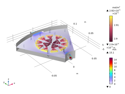
In the Settings window for 3D Plot Group, type Surface Species Concentration (sr) in the Label text field.
3
Locate the Data section. From the Dataset list, choose Study 2 - Rotating Insert Sections/Solution 2 (sol2).
4
From the Time (s) list, choose Last (90).
5
Locate the Plot Settings section. Clear the Plot dataset edges checkbox.
6
Locate the Color Legend section. Select the Show maximum and minimum values checkbox.
7
Select the Show units checkbox.
8
From the Position list, choose Right double.
9
Right-click Surface Species Concentration (sr) and choose Move Up.
Surface 1
1
Right-click Surface Species Concentration (sr) and choose Surface.
2
In the Settings window for Surface, locate the Expression section.
3
In the Expression text field, type cTiN.
4
Locate the Coloring and Style section. From the Color table list, choose Metasepia.
5
From the Color table transformation list, choose Reverse.
Arrow Volume 1
1
In the Model Builder window, right-click Surface Species Concentration (sr) and choose Arrow Volume.
2
In the Settings window for Arrow Volume, locate the Expression section.
3
In the x-component text field, type u.
4
In the y-component text field, type v.
5
In the z-component text field, type w.
6
Locate the Arrow Positioning section. Find the x grid points subsection. In the Points text field, type 5.
7
Find the y grid points subsection. In the Points text field, type 8.
8
Locate the Coloring and Style section. From the Arrow length list, choose Logarithmic.
9
In the Range quotient text field, type 500.
10
From the Color list, choose Custom.
11
12
Click Define custom colors.
13
14
Click Add to custom colors.
15
Click Show color palette only or OK on the cross-platform desktop.
Slice 1
1
Right-click Surface Species Concentration (sr) and choose Slice.
2
In the Settings window for Slice, locate the Expression section.
3
In the Expression text field, type spf.U.
4
Locate the Plane Data section. From the Plane list, choose xy-planes.
5
In the Planes text field, type 1.
Selection 1
1
Right-click Slice 1 and choose Selection.
2
Click in the Graphics window and then press Ctrl+A to select all domains.
Surface 2
1
In the Model Builder window, right-click Surface Species Concentration (sr) and choose Surface.
2
In the Settings window for Surface, locate the Data section.
3
From the Dataset list, choose Reactor Walls.
4
Locate the Expression section. In the Expression text field, type 1.
5
Locate the Coloring and Style section. From the Coloring list, choose Uniform.
6
From the Color list, choose Gray.
Contour 1
1
Right-click Surface Species Concentration (sr) and choose Contour.
2
In the Settings window for Contour, locate the Expression section.
3
In the Expression text field, type cTiN*chem.M_TiN_surf/rhoTiN.
4
Locate the Levels section. In the Total levels text field, type 10.
5
Locate the Coloring and Style section. From the Coloring list, choose Uniform.
6
From the Color list, choose White.
7
Clear the Color legend checkbox.
Average Deposition Layer Thickness
1
In the Model Builder window, right-click Average Deposition Rates and choose Duplicate.
2
In the Settings window for Evaluation Group, type Average Deposition Layer Thickness in the Label text field.
3
Locate the Data section. From the Dataset list, choose Study 2 - Rotating Insert Sections/Solution 2 (sol2).
4
Locate the Transformation section. In the Expression text field, type (av1-av4)/av1.
5
In the Column header text field, type (av1 - av4)/av1.
Surface Average 1
1
In the Model Builder window, expand the Average Deposition Layer Thickness node, then click Surface Average 1.
2
In the Settings window for Surface Average, locate the Expressions section.
3
Surface Average 2
1
In the Model Builder window, click Surface Average 2.
2
In the Settings window for Surface Average, locate the Expressions section.
3
Surface Average 3
1
In the Model Builder window, click Surface Average 3.
2
In the Settings window for Surface Average, locate the Expressions section.
3
Surface Average 4
1
In the Model Builder window, click Surface Average 4.
2
In the Settings window for Surface Average, locate the Expressions section.
3
Average Deposition Layer Thickness
1
In the Model Builder window, click Average Deposition Layer Thickness.
2
In the Average Deposition Layer Thickness toolbar, click  Evaluate.
Deposition Layer Thickness
1
In the Model Builder window, under Results > Rotating Insert Sections click Average Deposition Rate 1.
2
In the Settings window for 1D Plot Group, type Deposition Layer Thickness in the Label text field.
3
Locate the Plot Settings section.
4
Select the y-axis label checkbox. In the associated text field, type Deposition thickness (um).
5
Locate the Legend section. From the Position list, choose Middle right.
Table Graph 1
1
In the Model Builder window, expand the Deposition Layer Thickness node, then click Table Graph 1.
2
In the Settings window for Table Graph, locate the Data section.
3
From the Evaluation group list, choose Average Deposition Layer Thickness.
4
In the Columns list, choose Insert1 (um), Insert2 (um), Insert3 (um), and Insert4 (um).
5
Locate the Coloring and Style section. From the Width list, choose 2.
6
Find the Line markers subsection. From the Marker list, choose None.
Table Graph 2
1
In the Model Builder window, click Table Graph 2.
2
In the Settings window for Table Graph, locate the Data section.
3
From the Evaluation group list, choose Average Deposition Layer Thickness.
4
In the Columns list box, select (av1 - av4)/av1 (1).
5
Locate the Coloring and Style section. From the Width list, choose 2.
6
Find the Line markers subsection. From the Marker list, choose None.
7
In the Deposition Layer Thickness toolbar, click  Plot.
8
Click the  Zoom Extents button in the Graphics toolbar.