|
|
|


|
•
|
|
1.9·10-4
|
|||||
|
1.04·10-4
|
|||||
|
1.04·10-4
|
|
11.03 (10.9)
|
31.2 (30.4)
|
687 (678)
|
1.68 (1.67)
|
|
|
10.59 (10.65)
|
26.5 (25.6)
|
622 (611)
|
1.58 (1.55)
|
|
|
9.21 (9.79)
|
22.3 (26)
|
1003 (1084)
|
1.56 (1.63)
|

|
1
|
|
2
|
In the Select Physics tree, select Fluid Flow > Single-Phase Flow > Turbulent Flow > Turbulent Flow, Low Re k-ε (spf).
|
|
3
|
Click Add.
|
|
4
|
Click
|
|
5
|
In the Select Study tree, select Preset Studies for Selected Physics Interfaces > Stationary with Initialization.
|
|
6
|
Click
|
|
1
|
|
2
|
|
3
|
Click
|
|
4
|
Browse to the model’s Application Libraries folder and double-click the file turbulent_free_porous_parameters.txt.
|
|
1
|
|
2
|
|
3
|
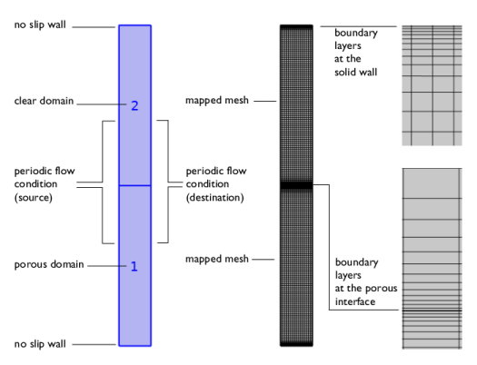
Select the Show geometry labels checkbox.
|
|
1
|
|
2
|
|
3
|
|
4
|
|
1
|
|
2
|
|
3
|
|
1
|
|
2
|
|
3
|
|
1
|
|
2
|
|
3
|
|
4
|
Click
|
|
1
|
|
2
|
|
3
|
|
1
|
|
2
|
|
3
|
|
4
|
|
5
|
Select the Snap to closest boundary checkbox.
|
|
1
|
In the Model Builder window, expand the Domain Point Probe 1 node, then click Point Probe Expression 1 (ppb1).
|
|
2
|
In the Settings window for Point Probe Expression, type Friction at the solid wall in the Label text field.
|
|
3
|
|
4
|
|
1
|
In the Model Builder window, under Component 1 (comp1) > Definitions right-click Domain Point Probe 1 and choose Duplicate.
|
|
2
|
|
3
|
|
1
|
In the Model Builder window, expand the Domain Point Probe 2 node, then click Friction at the solid wall (ppb2).
|
|
2
|
In the Settings window for Point Probe Expression, type Friction at the porous interface in the Label text field.
|
|
3
|
|
4
|
Locate the Expression section. In the Expression text field, type side(2,(spf.nuT+spf.nu)*pprint(uy)).
|
|
1
|
|
2
|
|
3
|
Click
|
|
4
|
Browse to the model’s Application Libraries folder and double-click the file turbulent_free_porous_variables.txt.
|
|
1
|
|
2
|
Go to the Add Material window.
|
|
3
|
|
4
|
Click the Add to Component button in the window toolbar.
|
|
5
|
|
6
|
|
7
|
|
8
|
Click OK.
|
|
1
|
|
2
|
Select the Enable porous media domains checkbox.
|
|
3
|
|
1
|
In the Model Builder window, under Component 1 (comp1) > Turbulent Flow, Low Re k-ε (spf) click Fluid Properties 1.
|
|
2
|
|
3
|
|
4
|
|
5
|
|
1
|
|
2
|
|
3
|
Specify the u vector as
|
|
1
|
|
1
|
|
2
|
|
3
|
|
4
|
|
1
|
|
2
|
|
3
|
|
4
|
|
5
|
|
1
|
|
3
|
|
4
|
|
5
|
|
1
|
|
3
|
|
4
|
|
1
|
|
2
|
|
3
|
|
1
|
|
3
|
|
4
|
|
1
|
|
3
|
|
4
|
|
1
|
|
3
|
|
4
|
|
1
|
|
2
|
|
3
|
Clear the Smooth transition to interior mesh checkbox.
|
|
1
|
In the Model Builder window, expand the Boundary Layers 1 node, then click Boundary Layer Properties.
|
|
3
|
|
4
|
|
5
|
|
6
|
|
7
|
|
1
|
In the Model Builder window, expand the Boundary Layers 2 node, then click Boundary Layer Properties.
|
|
3
|
|
4
|
|
5
|
|
6
|
|
7
|
Click
|
|
1
|
|
2
|
|
3
|
Click
|
|
5
|
Click
|
|
7
|
|
1
|
|
2
|
|
1
|
In the Model Builder window, under Study 1 > Solver Configurations click Parametric Solutions 1 - Copy 1 (sol7).
|
|
2
|
|
1
|
|
2
|
|
3
|
|
4
|
|
5
|
|
6
|
|
7
|
|
1
|
|
2
|
Click in the Graphics window and then press Ctrl+A to select both domains.
|
|
1
|
|
2
|
|
4
|
|
5
|
In the Dependent variable quantity table, enter the following settings:
|
|
6
|
Click
|
|
7
|
In the Source term quantity table, enter the following settings:
|
|
1
|
|
2
|
|
3
|
|
4
|
|
1
|
|
2
|
|
3
|
Click
|
|
4
|
Browse to the model’s Application Libraries folder and double-click the file turbulent_free_porous_parametric_study.txt.
|
|
1
|
|
2
|
|
1
|
|
2
|
|
3
|
|
1
|
|
2
|
|
4
|
|
5
|
|
6
|
Browse to the model’s Application Libraries folder and double-click the file turbulent_free_porous_U_E95.txt.
|
|
1
|
|
2
|
|
3
|
|
4
|
Browse to the model’s Application Libraries folder and double-click the file turbulent_free_porous_k_E95.txt.
|
|
1
|
|
2
|
|
3
|
|
4
|
Browse to the model’s Application Libraries folder and double-click the file turbulent_free_porous_uv_E95.txt.
|
|
1
|
|
2
|
|
3
|
|
4
|
Browse to the model’s Application Libraries folder and double-click the file turbulent_free_porous_U_#06_5400.txt.
|
|
1
|
|
2
|
|
3
|
|
4
|
Browse to the model’s Application Libraries folder and double-click the file turbulent_free_porous_uv_#06_5400.txt.
|
|
1
|
|
2
|
|
3
|
|
4
|
Browse to the model’s Application Libraries folder and double-click the file turbulent_free_porous_U_#06_9500.txt.
|
|
1
|
|
2
|
|
3
|
|
4
|
Browse to the model’s Application Libraries folder and double-click the file turbulent_free_porous_uv_#06_9500.txt.
|
|
1
|
|
2
|
|
3
|
|
4
|
Browse to the model’s Application Libraries folder and double-click the file turbulent_free_porous_rms_#06.txt.
|
|
1
|
|
2
|
|
3
|
|
4
|
|
5
|
Locate the Data Column Settings section. In the table, click to select the cell at row number 2 and column number 1.
|
|
6
|
|
1
|
|
2
|
|
3
|
Locate the Data Column Settings section. In the table, enter the following settings:
|
|
4
|
|
1
|
|
2
|
|
3
|
Locate the Data Column Settings section. In the table, enter the following settings:
|
|
4
|
|
1
|
|
2
|
|
3
|
Locate the Data Column Settings section. In the table, enter the following settings:
|
|
4
|
|
1
|
|
2
|
|
3
|
|
4
|
|
1
|
|
2
|
|
3
|
|
4
|
|
5
|
In the Parameter values (ReH,H (m),epsilon_p_i,cF_i,Da_i) list box, select 1: ReH=5500, H=0.03 m, epsilon_p_i=0.95, cF_i=0.14, Da_i=1.9E-4.
|
|
6
|
|
7
|
|
8
|
Locate the Plot Settings section.
|
|
9
|
|
10
|
|
11
|
|
12
|
|
13
|
|
14
|
|
15
|
|
1
|
|
2
|
|
3
|
|
4
|
|
5
|
|
6
|
|
7
|
|
8
|
|
9
|
|
10
|
Select the Label checkbox.
|
|
1
|
|
2
|
|
3
|
|
4
|
|
5
|
|
6
|
|
7
|
|
1
|
|
2
|
|
3
|
|
4
|
Locate the Coloring and Style section. Find the Line style subsection. From the Line list, choose None.
|
|
5
|
|
6
|
|
7
|
|
8
|
|
9
|
Select the Label checkbox.
|
|
1
|
|
2
|
|
3
|
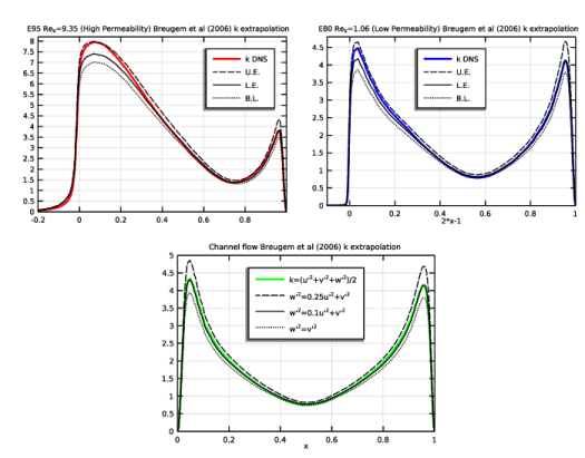
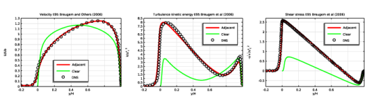
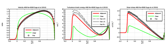
Locate the Title section. In the Title text area, type Turbulence kinetic energy E95 Breugem et al (2006).
|
|
4
|
Locate the Plot Settings section. In the y-axis label text field, type k/u<sup>s</sup><sub>\tau</sub> <sup>2</sup>.
|
|
5
|
|
6
|
|
1
|
|
2
|
|
3
|
|
1
|
|
2
|
|
3
|
|
1
|
|
2
|
|
3
|
|
4
|
Locate the Coloring and Style section. Find the Line markers subsection. From the Positioning list, choose Interpolated.
|
|
5
|
|
1
|
|
2
|
|
3
|
|
4
|
|
5
|
Locate the Plot Settings section. In the y-axis label text field, type -u<sup>\prime</sup>v<sup>\prime</sup>/u<sup>s</sup><sub>\tau</sub> <sup>2</sup>.
|
|
6
|
|
7
|
|
8
|
|
1
|
|
2
|
|
3
|
|
1
|
|
2
|
|
3
|
|
1
|
|
2
|
|
3
|
|
1
|
|
2
|
|
3
|
Locate the Data section. In the Parameter values (ReH,H (m),epsilon_p_i,cF_i,Da_i) list box, select 2: ReH=5400, H=0.029 m, epsilon_p_i=0.8, cF_i=0.095, Da_i=1.04E-4.
|
|
4
|
|
1
|
|
2
|
|
3
|
|
1
|
|
2
|
|
3
|
|
1
|
|
2
|
|
3
|
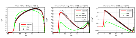
Locate the Data section. In the Parameter values (ReH,H (m),epsilon_p_i,cF_i,Da_i) list box, select 2: ReH=5400, H=0.029 m, epsilon_p_i=0.8, cF_i=0.095, Da_i=1.04E-4.
|
|
4
|
Locate the Title section. In the Title text area, type Turbulence kinetic energy #06 Re=5400 Suga et al (2010).
|
|
1
|
|
2
|
|
3
|
|
1
|
|
2
|
|
3
|
Locate the y-Axis Data section. In the Expression text field, type ((1+cUu)*u1(x)^2+(1+cUv)*v1(x)^2)/2.
|
|
4
|
|
5
|
Locate the Coloring and Style section. Find the Line style subsection. From the Line list, choose Dashed.
|
|
6
|
|
7
|
|
8
|
|
1
|
|
2
|
|
3
|
Locate the y-Axis Data section. In the Expression text field, type ((1+cLu)*u1(x)^2+(1+cLv)*v1(x)^2)/2.
|
|
4
|
Locate the Coloring and Style section. Find the Line style subsection. From the Line list, choose Solid.
|
|
5
|
Locate the Legends section. In the table, enter the following settings:
|
|
1
|
|
2
|
|
3
|
|
4
|
Locate the Coloring and Style section. Find the Line style subsection. From the Line list, choose Dotted.
|
|
5
|
Locate the Legends section. In the table, enter the following settings:
|
|
1
|
|
2
|
|
3
|
Locate the Data section. In the Parameter values (ReH,H (m),epsilon_p_i,cF_i,Da_i) list box, select 2: ReH=5400, H=0.029 m, epsilon_p_i=0.8, cF_i=0.095, Da_i=1.04E-4.
|
|
4
|
|
1
|
|
2
|
|
3
|
|
1
|
|
2
|
|
3
|
|
1
|
|
2
|
|
3
|
Locate the Data section. In the Parameter values (ReH,H (m),epsilon_p_i,cF_i,Da_i) list box, select 3: ReH=9500, H=0.029 m, epsilon_p_i=0.8, cF_i=0.095, Da_i=1.04E-4.
|
|
4
|
|
1
|
|
2
|
|
3
|
|
1
|
|
2
|
|
3
|
|
1
|
|
2
|
|
3
|
Locate the Data section. In the Parameter values (ReH,H (m),epsilon_p_i,cF_i,Da_i) list box, select 3: ReH=9500, H=0.029 m, epsilon_p_i=0.8, cF_i=0.095, Da_i=1.04E-4.
|
|
4
|
Locate the Title section. In the Title text area, type Turbulence kinetic energy #06 Re=9500 Suga et al (2010).
|
|
1
|
|
2
|
|
3
|
|
1
|
|
2
|
|
3
|
|
1
|
|
2
|
|
3
|
|
1
|
|
2
|
|
3
|
|
1
|
|
2
|
|
3
|
Locate the Data section. In the Parameter values (ReH,H (m),epsilon_p_i,cF_i,Da_i) list box, select 3: ReH=9500, H=0.029 m, epsilon_p_i=0.8, cF_i=0.095, Da_i=1.04E-4.
|
|
4
|
|
1
|
|
2
|
|
3
|
|
1
|
|
2
|
|
3
|
|
1
|
|
2
|
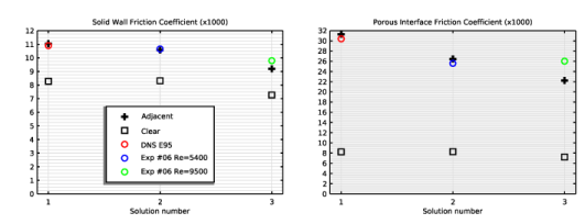
In the Settings window for 1D Plot Group, type Solid Wall Friction Coefficient (x1000) in the Label text field.
|
|
3
|
|
4
|
|
5
|
|
6
|
|
7
|
|
8
|
|
9
|
|
10
|
|
11
|
|
1
|
|
2
|
|
3
|
|
4
|
Locate the y-Axis Data section. In the table, enter the following settings:
|
|
5
|
Click to expand the Coloring and Style section. Find the Line style subsection. From the Line list, choose None.
|
|
6
|
|
7
|
|
8
|
|
9
|
Clear the Solution checkbox.
|
|
10
|
Select the Label checkbox.
|
|
1
|
|
2
|
|
3
|
|
4
|
Locate the Coloring and Style section. Find the Line markers subsection. From the Marker list, choose Square.
|
|
1
|
|
2
|
|
3
|
Locate the Data section. From the Parameter selection (ReH, H, epsilon_p_i, cF_i, Da_i) list, choose From list.
|
|
4
|
In the Parameter values (ReH,H (m),epsilon_p_i,cF_i,Da_i) list box, select 1: ReH=5500, H=0.03 m, epsilon_p_i=0.95, cF_i=0.14, Da_i=1.9E-4.
|
|
5
|
Locate the y-Axis Data section. In the table, enter the following settings:
|
|
6
|
|
7
|
|
1
|
|
2
|
|
3
|
Locate the Data section. In the Parameter values (ReH,H (m),epsilon_p_i,cF_i,Da_i) list box, select 2: ReH=5400, H=0.029 m, epsilon_p_i=0.8, cF_i=0.095, Da_i=1.04E-4.
|
|
4
|
Locate the y-Axis Data section. In the table, enter the following settings:
|
|
5
|
|
1
|
|
2
|
|
3
|
Locate the Data section. In the Parameter values (ReH,H (m),epsilon_p_i,cF_i,Da_i) list box, select 3: ReH=9500, H=0.029 m, epsilon_p_i=0.8, cF_i=0.095, Da_i=1.04E-4.
|
|
4
|
|
5
|
Locate the y-Axis Data section. In the table, enter the following settings:
|
|
1
|
In the Model Builder window, right-click Solid Wall Friction Coefficient (x1000) and choose Annotation.
|
|
2
|
|
3
|
In the Text text field, type Sol 1: E95 \\ Re=5500 \\ $\epsilon_p=0.95$ \\ Da=1.9e-4 \\ $c_F=0.14$ \\ ~ \\ Sol 2: #06 Re=5400 \\ Sol 3: #06 Re=9500 \\ $\epsilon_p$=0.8 \\ Da=1.04e-4 \\ $c_F=0.095$.
|
|
4
|
Select the LaTeX markup checkbox.
|
|
5
|
|
6
|
|
7
|
|
8
|
|
9
|
Select the Show frame checkbox.
|
|
10
|
|
1
|
|
2
|
In the Settings window for 1D Plot Group, type Porous Interface Friction Coefficient (x1000) in the Label text field.
|
|
3
|
Click to expand the Title section. In the Title text area, type Porous Interface Friction Coefficient (x1000).
|
|
4
|
|
1
|
In the Model Builder window, expand the Porous Interface Friction Coefficient (x1000) node, then click Adjacent.
|
|
2
|
|
1
|
|
2
|
|
1
|
|
2
|
|
1
|
|
2
|
|
1
|
|
2
|
|
1
|
|
2
|
|
3
|
|
1
|
In the Model Builder window, right-click Porous Interface Friction Coefficient (x1000) and choose Duplicate.
|
|
2
|
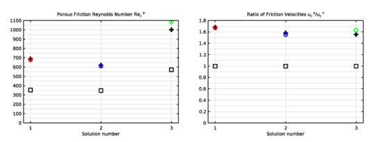
In the Settings window for 1D Plot Group, type Porous Friction Reynolds Number in the Label text field.
|
|
3
|
Click to expand the Title section. In the Title text area, type Porous Friction Reynolds Number Re<sub>\tau</sub> <sup>p</sup>.
|
|
4
|
|
5
|
|
1
|
|
2
|
|
1
|
|
2
|
|
1
|
|
2
|
|
1
|
|
2
|
|
1
|
|
2
|
|
1
|
|
2
|
|
3
|
|
1
|
|
2
|
In the Settings window for 1D Plot Group, type Ratio of Friction Velocities in the Label text field.
|
|
3
|
Click to expand the Title section. In the Title text area, type Ratio of Friction Velocities u<sub>\tau</sub> <sup>p</sup>/u<sub>\tau</sub> <sup>s</sup>.
|
|
4
|
|
5
|
|
1
|
|
2
|
|
1
|
|
2
|
|
1
|
|
2
|
|
1
|
|
2
|
|
1
|
|
2
|
|
1
|
|
2
|
|
3
|
|
1
|
|
2
|
|
3
|
|
4
|
From the Parameter value (ReH,H (m),epsilon_p_i,cF_i,Da_i) list, choose 1: ReH=5500, H=0.03 m, epsilon_p_i=0.95, cF_i=0.14, Da_i=1.9E-4.
|
|
5
|
|
6
|
|
7
|
|
8
|
|
9
|
|
1
|
|
2
|
|
3
|
|
4
|
|
5
|
Locate the Arrow Positioning section. Find the x grid points subsection. In the Points text field, type 1.
|
|
6
|
|
7
|
|
8
|
|
1
|
|
2
|
|
3
|
|
1
|
|
2
|
|
3
|
|
4
|
|
1
|
In the Model Builder window, expand the Turbulence kinetic energy node, then click Color Expression 1.
|
|
2
|
|
3
|
|
1
|
|
2
|
|
3
|
|
4
|
|
1
|
|
2
|
|
3
|
|
1
|
|
2
|
|
3
|
Select the LaTeX markup checkbox.
|
|
4
|
|
5
|
|
6
|
|
7
|
|
8
|
|
9
|
|
1
|
|
2
|
|
3
|
|
4
|
|
1
|
|
2
|
|
3
|
|
4
|
|
5
|
|
1
|
|
2
|
|
3
|
|
4
|
Locate the Expressions section. In the table, enter the following settings:
|
|
1
|
|
2
|
|
3
|