PDF

Squeeze Film Between Rectangular Porous and Nonporous Plates
Introduction
This example describes how to simulate the flow of a thin film of fluid in the gap between two rectangular plates, one of them with a porous facing, when the fluid is squeezed as a consequence of the relative motion between the plates. The model accounts for the ingress and egress of fluid between the porous material and the thin-film region. The simple geometry of the model allows for the comparison of the computed solution with analytic expressions in Ref. 1.
Model Definition
The model is set up with parameterized quantities in a unitless base system. It uses a thin-film flow approximation, described by the Reynolds equation, for the fluid motion in the gap between the plates. The fluid flow in the porous region is described by Darcy’s law. The coupling between the Thin-Film Flow interface and the Darcy’s Law interface is handled by the Thin-Film and Porous Media multiphysics coupling.
Geometry
The length of the rectangular plates, a, is taken to be of unit value. The width, b is controlled by the aspect ratio parameter, k = a/b. Using symmetry planes orthogonal to the x- and y-axes, only one quarter of the plate is modeled, as shown in  Figure 1. The height of the porous facing, H, is suitably scaled with respect to the plate length using the parameter,  = H/a. A rigid body motion is considered for the nonporous plate and it is therefore not included in the model geometry. The relative motion between the porous and nonporous plates can be accounted for by the motion of the “wall” or “base” defined in the Thin-Film Flow interface.
Figure 1: Computational domain with symmetry boundaries (in yellow) and the thin-film region (in purple).
Physics Interface Settings
The Thin-Film Flow interface is set up to solve the Reynolds equation. The reference pressure, pref, is set to zero. The parameterized fluid density, ρ, and viscosity, η, are both set to unit value. The thin-film thickness is chosen to be, ht = 0.001, and set as the height of the wall above the reference plane. The squeeze action is induced by applying a wall velocity in the positive z direction of unit magnitude controlled by the parameter, vsq. Symmetry condition is applied to edges corresponding to the symmetry boundaries in the geometry. Border condition with zero pressure is applied to other edges as default.
The Darcy’s Law interface is set up with zero reference pressure and similar fluid properties to that in the Thin-Film Flow interface. The porosity, εp, is set to zero and the permeability, , is chosen to be isotropic in nature, with a value controlled by the permeability parameter, . The boundary conditions include a No Flow condition on the top face, a Symmetry condition on the symmetry boundaries, and a Pressure condition with zero prescribed value elsewhere.
The multiphysics coupling, added automatically, acts at the intersection of the two interfaces. It accounts for the fluid motion and the pressure balance in the region.
Meshing
A structured mesh with hexahedral elements is constructed using the Mapped and Swept mesh features. The porous domain thickness is meshed with four elements. The resulting mesh is shown in Figure 2.
Figure 2: Computational domain with structured, hexahedral mesh.
Results and Discussion
The analysis presented in Ref. 1 provides the expression for the dimensionless pressure at the intersection of the physics interfaces. It is given in the form of infinite series as
(1),
where
(2),
(3),
(4),
(5).
The dimensionless load carrying capacity of the squeeze film is given as
(6).
In the comparison plots presented in the following paragraphs, the values of m and n are taken to be equal to 29, as suggested in Ref. 1. This ensures accurate pressure and load capacity values up to five significant digits.
Figure 3 shows pressure distribution for different values of ψ on the intersecting boundary of the physics interfaces at the location y = b/2, for values k = 1 and  = 0.02. The maximum pressure rapidly decreases with an increase in the permeability parameter. For values of ψ < 0.001, the behavior is close to the nonporous limit as reported in Ref. 1.
Figure 3: Pressure distribution for various values of ψ.
Figure 4 shows the load capacity for different values of k at the intersecting boundary of the physics interfaces for the value of  = 0.02. The load-carrying capacity generally decreases with an increase in the aspect ratio, as such plates cannot contain the pressure generated due to increased side leakage. In fact, square plates provide the highest load-bearing capacity for a given quadrilateral area of coverage.
Figure 4: Load capacity for various values of k.
Figure 5 shows the loss of load capacity with increasing aspect ratio and permeability parameter.
Figure 5: Load capacity for various values of ψ.
Figure 6 shows load capacity for different values of at the intersection of the physics interfaces for the values of k = 1 and ht = 0.001. The load capacity is large and shows little variation with changes in the porous domain thickness for low permeabilities.With an increase in the permeability and porous domain thickness, however, the load capacity rapidly deteriorates.
Figure 6: Load capacity for various values of .
All comparison plots show excellent agreement between computed and analytic solutions.
Figure 7 shows the pressure developed at the intersection of the physics interfaces and the subsequent percolation flow in the porous domain as a consequence of the squeezing action of the plates on the fluid in the thin-film region for the case k = 1,  = 0.02, and ψ = 0.01.
Figure 7: Darcy pressure and velocity streamlines.
Reference
1. H. Wu, “An Analysis of the Squeeze Film Between Porous Rectangular Plates,” J. Lubr. Technol., vol. 94, no. 1, pp. 64–68, 1972.
Application Library path: CFD_Module/Verification_Examples/squeeze_film_porous
Modeling Instructions
From the File menu, choose New.
New
In the New window, click  Model Wizard.
Model Wizard
1
In the Model Wizard window, click  3D.
2
In the Select Physics tree, select Fluid Flow > Porous Media and Subsurface Flow > Thin-Film and Porous Media Flow.
3
Click Add.
4
Click  Study.
5
In the Select Study tree, select General Studies > Stationary.
6
Choose a unitless base system.
Root
1
In the Model Builder window, click the root node.
2
In the root node’s Settings window, locate the Unit System section.
3
From the Unit system list, choose None.
Global Definitions
Parameters 1
1
In the Model Builder window, under Global Definitions click Parameters 1.
2
In the Settings window for Parameters, locate the Parameters section.
3
Click  Load from File.
4
Define analytic expressions of the solution. The expressions are available in Equation 1Equation 6.
Definitions
Analytic 1 (an1)
1
In the Definitions toolbar, click  Analytic.
2
In the Settings window for Analytic, type a_m in the Function name text field.
3
Locate the Definition section. In the Expression text field, type m*pi/a.
4
In the Arguments text field, type m, a.
5
Locate the Plot Parameters section. In the table, enter the following settings:
Analytic 2 (an2)
1
In the Definitions toolbar, click  Analytic.
2
In the Settings window for Analytic, type b_n in the Function name text field.
3
Locate the Definition section. In the Expression text field, type n*pi/b.
4
In the Arguments text field, type n, b.
5
Locate the Plot Parameters section. In the table, enter the following settings:
Analytic 3 (an3)
1
In the Definitions toolbar, click  Analytic.
2
In the Settings window for Analytic, type gamma_mn in the Function name text field.
3
Locate the Definition section. In the Expression text field, type pi*sqrt(m^2+(k*n)^2)/a.
4
In the Arguments text field, type m, n, k, a.
5
Locate the Plot Parameters section. In the table, enter the following settings:
Analytic 4 (an4)
1
In the Definitions toolbar, click  Analytic.
2
In the Settings window for Analytic, type G_mn in the Function name text field.
3
Locate the Definition section. In the Expression text field, type 12*(exp(2*gamma_mn*H)-1)/(H*(exp(2*gamma_mn*H)+1)/a).
4
In the Arguments text field, type gamma_mn, H, a.
5
Locate the Plot Parameters section. In the table, enter the following settings:
Analytic 5 (an5)
1
In the Definitions toolbar, click  Analytic.
2
In the Settings window for Analytic, type p_summand in the Function name text field.
3
Locate the Definition section. In the Expression text field, type (sin(a_m((2*m-1),a)*x)*sin(b_n((2*n-1),b)*y))/((2*m-1)*(2*n-1)*sqrt((2*m-1)^2+(k*(2*n-1))^2)*(pi*sqrt((2*m-1)^2+(k*(2*n-1))^2)+(psi*G_mn(gamma_mn((2*m-1),(2*n-1),k,a),H,a)))).
4
In the Arguments text field, type m, n, x, y, a, b, psi, k, H.
5
Locate the Plot Parameters section. In the table, enter the following settings:
Analytic 6 (an6)
1
In the Definitions toolbar, click  Analytic.
2
In the Settings window for Analytic, type W_summand_psi in the Function name text field.
3
Locate the Definition section. In the Expression text field, type 1/(((2*m-1)*(2*n-1))^2*sqrt((2*m-1)^2+(k*(2*n-1))^2)*((pi*sqrt((2*m-1)^2+(k*(2*n-1))^2))+(psi*G_mn(gamma_mn((2*m-1),(2*n-1),k,a),H,a)))).
4
In the Arguments text field, type m, n, a, psi, k, H.
5
Locate the Plot Parameters section. In the table, enter the following settings:
Analytic 7 (an7)
1
In the Definitions toolbar, click  Analytic.
2
In the Settings window for Analytic, type W_summand_phi in the Function name text field.
3
Locate the Definition section. In the Expression text field, type 1/(((2*m-1)*(2*n-1))^2*sqrt((2*m-1)^2+(k*(2*n-1))^2)*((pi*sqrt((2*m-1)^2+(k*(2*n-1))^2))+(phi*H/ht^3*G_mn(gamma_mn((2*m-1),(2*n-1),k,a),H,a)))).
4
In the Arguments text field, type m, n, a, phi, k, H.
5
Locate the Plot Parameters section. In the table, enter the following settings:
Geometry 1
Block 1 (blk1)
1
In the Geometry toolbar, click  Block.
2
In the Settings window for Block, locate the Size and Shape section.
3
In the Width text field, type a/2.
4
In the Depth text field, type b/2.
5
In the Height text field, type H.
Form Union (fin)
In the Geometry toolbar, click  Build All.
Create selections for the thin-film domain and symmetry boundaries.
Definitions
Thin-Film Boundary
1
In the Definitions toolbar, click  Explicit.
2
In the Settings window for Explicit, type Thin-Film Boundary in the Label text field.
3
Locate the Input Entities section. From the Geometric entity level list, choose Boundary.
4
Click  Paste Selection.
5
In the Paste Selection dialog, type 3 in the Selection text field.
6
7
In the Settings window for Explicit, locate the Color section.
8
From the Color list, choose Color 1.
Symmetry Boundaries
1
In the Definitions toolbar, click  Explicit.
2
In the Settings window for Explicit, type Symmetry Boundaries in the Label text field.
3
Locate the Input Entities section. From the Geometric entity level list, choose Boundary.
4
Click  Paste Selection.
5
In the Paste Selection dialog, type 5-6 in the Selection text field.
6
7
In the Settings window for Explicit, locate the Color section.
8
From the Color list, choose Color 4.
9
Click the  Show Grid button in the Graphics toolbar.
10
Click the  Zoom Extents button in the Graphics toolbar.
Next, specify parameters for the Thin-Film Flow interface: Set the reference pressure to zero and reverse the reference normal to point in the positive z direction.
Thin-Film Flow (tff)
1
In the Model Builder window, under Component 1 (comp1) click Thin-Film Flow (tff).
2
In the Settings window for Thin-Film Flow, locate the Boundary Selection section.
3
From the Selection list, choose Thin-Film Boundary.
4
Locate the Reference Pressure section. In the pref text field, type 0.
Fluid-Film Properties 1
1
In the Model Builder window, under Component 1 (comp1) > Thin-Film Flow (tff) click Fluid-Film Properties 1.
2
In the Settings window for Fluid-Film Properties, locate the Model Input section.
3
From the T list, choose Common model input.
4
Click to expand the Reference Surface Properties section. From the Reference normal orientation list, choose Opposite direction to geometry normal.
5
Locate the Wall Properties section. In the hw1 text field, type ht.
6
From the vw list, choose User defined. Specify the vector as
7
Locate the Fluid Properties section. From the μ list, choose User defined. In the associated text field, type eta.
8
From the ρ list, choose User defined. In the associated text field, type rho.
Symmetry 1
1
In the Physics toolbar, click  Edges and choose Symmetry.
2
In the Settings window for Symmetry, locate the Edge Selection section.
3
Click  Paste Selection.
4
In the Paste Selection dialog, type 7, 10 in the Selection text field.
5
Now specify parameters for the Darcy’s Law interface, including a zero reference pressure.
Darcy’s Law (dl)
1
In the Model Builder window, under Component 1 (comp1) click Darcy’s Law (dl).
2
In the Settings window for Darcy’s Law, locate the Physical Model section.
3
In the pref text field, type 0.
Fluid 1
1
In the Model Builder window, under Component 1 (comp1) > Darcy’s Law (dl) > Porous Medium 1 click Fluid 1.
2
In the Settings window for Fluid, locate the Fluid Properties section.
3
From the ρ list, choose User defined. In the associated text field, type rho.
4
From the μ list, choose User defined. In the associated text field, type eta.
Porous Matrix 1
1
In the Model Builder window, click Porous Matrix 1.
2
In the Settings window for Porous Matrix, locate the Matrix Properties section.
3
From the εp list, choose User defined. From the κ list, choose User defined. In the associated text field, type phi.
Symmetry 1
1
In the Physics toolbar, click  Boundaries and choose Symmetry.
2
In the Settings window for Symmetry, locate the Boundary Selection section.
3
From the Selection list, choose Symmetry Boundaries.
Pressure 1
1
In the Physics toolbar, click  Boundaries and choose Pressure.
2
In the Settings window for Pressure, locate the Boundary Selection section.
3
Click  Paste Selection.
4
In the Paste Selection dialog, type 1, 2 in the Selection text field.
5
Create a structured hexahedral mesh.
Mesh 1
1
In the Model Builder window, under Component 1 (comp1) click Mesh 1.
2
In the Settings window for Mesh, locate the Physics-Controlled Mesh section.
3
From the Element size list, choose Extremely fine.
4
Locate the Sequence Type section. From the list, choose User-controlled mesh.
Mapped 1
1
In the Mesh toolbar, click  More Generators and choose Mapped.
2
In the Settings window for Mapped, locate the Boundary Selection section.
3
From the Selection list, choose Thin-Film Boundary.
Swept 1
In the Mesh toolbar, click  Swept.
Distribution 1
1
Right-click Swept 1 and choose Distribution.
2
In the Settings window for Distribution, locate the Distribution section.
3
In the Number of elements text field, type 4.
Free Tetrahedral 1
1
In the Model Builder window, under Component 1 (comp1) > Mesh 1 right-click Free Tetrahedral 1 and choose Disable.
2
Right-click Mesh 1 and choose Build All.
3
Click the  Zoom Extents button in the Graphics toolbar.
Study 1
1
In the Model Builder window, click Study 1.
2
In the Settings window for Study, locate the Study Settings section.
3
Clear the Generate default plots checkbox.
Add a Parametric Sweep step for computing the Stationary solution for specified parameter combinations.
Parametric Sweep
1
In the Study toolbar, click  Parametric Sweep.
2
In the Settings window for Parametric Sweep, locate the Study Settings section.
3
4
5
6
7
8
9
In the Study toolbar, click  Compute.
Results
1
In the Model Builder window, click Results.
2
In the Settings window for Results, locate the Update of Results section.
3
Select the Only plot when requested checkbox.
Prepare datasets for processing the results and analytic functions.
Mirror 3D 1
1
In the Model Builder window, expand the Results node.
2
Right-click Results > Datasets and choose More 3D Datasets > Mirror 3D.
3
In the Settings window for Mirror 3D, locate the Data section.
4
From the Dataset list, choose Study 1/Parametric Solutions 1 (sol2).
5
Locate the Plane Data section. From the Plane list, choose XZ-planes.
6
In the Y-coordinate text field, type b/2.
Mirror 3D 2
1
In the Results toolbar, click  More Datasets and choose Mirror 3D.
2
In the Settings window for Mirror 3D, locate the Plane Data section.
3
In the X-coordinate text field, type a/2.
4
Locate the Data section. From the Dataset list, choose Mirror 3D 1.
Cut Line 3D 1
1
In the Results toolbar, click  Cut Line 3D.
2
In the Settings window for Cut Line 3D, locate the Data section.
3
From the Dataset list, choose Mirror 3D 2.
4
Locate the Line Data section. In row Point 1, set y to b/2.
5
In row Point 2, set x to a.
6
In row Point 2, set y to b/2.
Grid 1D 1
1
In the Results toolbar, click  More Datasets and choose Grid > Grid 1D.
2
In the Settings window for Grid 1D, locate the Data section.
3
From the Source list, choose Function.
4
From the Function list, choose All.
5
Locate the Parameter Bounds section. In the Name text field, type psi.
6
In the Minimum text field, type 1e-4.
Grid 1D 2
1
In the Results toolbar, click  More Datasets and choose Grid > Grid 1D.
2
In the Settings window for Grid 1D, locate the Data section.
3
From the Source list, choose Function.
4
From the Function list, choose All.
5
Locate the Parameter Bounds section. In the Name text field, type k.
6
In the Minimum text field, type 1.
7
In the Maximum text field, type 8.
Grid 1D 3
1
In the Results toolbar, click  More Datasets and choose Grid > Grid 1D.
2
In the Settings window for Grid 1D, locate the Data section.
3
From the Source list, choose Function.
4
From the Function list, choose All.
5
Locate the Parameter Bounds section. In the Name text field, type H.
6
In the Minimum text field, type 0.02.
7
In the Maximum text field, type 0.1.
Compute the load capacity for different parameter values.
Surface Integration 1
1
In the Results toolbar, click  More Derived Values and choose Integration > Surface Integration.
2
In the Settings window for Surface Integration, locate the Data section.
3
From the Dataset list, choose Mirror 3D 2.
4
From the Parameter selection (k, psi, Hbar) list, choose Manual.
5
In the Parameter indices (1-35) text field, type range(1,1,5).
6
Locate the Selection section. From the Selection list, choose Thin-Film Boundary.
7
Locate the Expressions section. In the table, enter the following settings:
Surface Integration 2
1
Right-click Surface Integration 1 and choose Duplicate.
2
In the Settings window for Surface Integration, locate the Data section.
3
In the Parameter indices (1-35) text field, type range(5,1,10).
Surface Integration 3
1
Right-click Surface Integration 2 and choose Duplicate.
2
In the Settings window for Surface Integration, locate the Data section.
3
In the Parameter indices (1-35) text field, type range(10,1,15).
Surface Integration 4
1
Right-click Surface Integration 3 and choose Duplicate.
2
In the Settings window for Surface Integration, locate the Data section.
3
In the Parameter indices (1-35) text field, type range(15,1,20).
Surface Integration 5
1
Right-click Surface Integration 4 and choose Duplicate.
2
In the Settings window for Surface Integration, locate the Data section.
3
In the Parameter indices (1-35) text field, type range(1,5,20).
Surface Integration 6
1
Right-click Surface Integration 5 and choose Duplicate.
2
In the Settings window for Surface Integration, locate the Data section.
3
In the Parameter indices (1-35) text field, type range(2,5,20).
Surface Integration 7
1
Right-click Surface Integration 6 and choose Duplicate.
2
In the Settings window for Surface Integration, locate the Data section.
3
In the Parameter indices (1-35) text field, type range(3,5,20).
Surface Integration 8
1
Right-click Surface Integration 7 and choose Duplicate.
2
In the Settings window for Surface Integration, locate the Data section.
3
In the Parameter indices (1-35) text field, type range(4,5,20).
Surface Integration 9
1
Right-click Surface Integration 8 and choose Duplicate.
2
In the Settings window for Surface Integration, locate the Data section.
3
In the Parameter indices (1-35) text field, type range(21,1,25).
Surface Integration 10
1
Right-click Surface Integration 9 and choose Duplicate.
2
In the Settings window for Surface Integration, locate the Data section.
3
In the Parameter indices (1-35) text field, type range(26,1,30).
Surface Integration 11
1
Right-click Surface Integration 10 and choose Duplicate.
2
In the Settings window for Surface Integration, locate the Data section.
3
In the Parameter indices (1-35) text field, type range(31,1,35).
4
In the Results toolbar, click  Evaluate and choose Clear and Evaluate All.
Pressure Distribution for Various psi Values
1
In the Results toolbar, click  1D Plot Group.
2
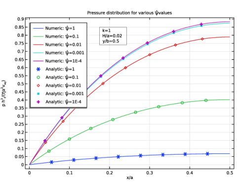
In the Settings window for 1D Plot Group, type Pressure Distribution for Various psi Values in the Label text field.
3
Locate the Data section. From the Dataset list, choose Cut Line 3D 1.
4
From the Parameter selection (k, psi, Hbar) list, choose From list.
5
In the Parameter values (k,psi,Hbar) list, choose 16: k=1, psi=1, Hbar=0.02, 17: k=1, psi=0.1, Hbar=0.02, 18: k=1, psi=0.01, Hbar=0.02, 19: k=1, psi=0.001, Hbar=0.02, and 20: k=1, psi=1E-4, Hbar=0.02.
6
Click to expand the Title section. From the Title type list, choose Manual.
7
In the Title text area, type Pressure distribution for various \psi values.
8
Locate the Plot Settings section.
9
Select the x-axis label checkbox. In the associated text field, type x/a.
10
Select the y-axis label checkbox. In the associated text field, type p h<sup>3</sup><sub>t</sub>/(\eta a<sup>2</sup>v<sub>sq</sub>).
11
Locate the Legend section. From the Position list, choose Upper left.
Line Graph 1
1
Right-click Pressure Distribution for Various psi Values and choose Line Graph.
2
In the Settings window for Line Graph, locate the y-Axis Data section.
3
In the Expression text field, type p*ht^3/(eta*a^2*sqvel).
4
Locate the x-Axis Data section. From the Parameter list, choose Expression.
5
In the Expression text field, type x/a.
6
Click to expand the Coloring and Style section. Click to expand the Legends section. Select the Show legends checkbox.
7
From the Legends list, choose Manual.
8
Line Graph 2
1
In the Model Builder window, right-click Pressure Distribution for Various psi Values and choose Line Graph.
2
In the Settings window for Line Graph, locate the y-Axis Data section.
3
In the Expression text field, type 192*sum(sum(p_summand(m, n, x, y, a, b, psi, 1, 0.02), n, 1, 15), m, 1, 15)/(pi^3).
4
Locate the x-Axis Data section. From the Parameter list, choose Expression.
5
In the Expression text field, type x/a.
6
Locate the Coloring and Style section. From the Color list, choose Cycle (reset).
7
Find the Line markers subsection. From the Marker list, choose Cycle (reset).
8
Find the Line style subsection. From the Line list, choose None.
9
Find the Line markers subsection. From the Positioning list, choose Interpolated.
10
Locate the Legends section. Select the Show legends checkbox.
11
From the Legends list, choose Manual.
12
Annotation 1
1
Right-click Pressure Distribution for Various psi Values and choose Annotation.
2
In the Settings window for Annotation, locate the Annotation section.
3
In the Text text field, type k=eval(k) \\ H/a=eval(Hbar) \\ y/b=0.5.
4
Select the LaTeX markup checkbox.
5
Locate the Position section. In the x text field, type 0.175.
6
In the y text field, type 0.85.
7
Click to expand the Advanced section. In the Precision text field, type 1.
8
Locate the Coloring and Style section. Clear the Show point checkbox.
9
Select the Show frame checkbox.
Pressure Distribution for Various psi Values
1
In the Model Builder window, click Pressure Distribution for Various psi Values.
2
In the Pressure Distribution for Various psi Values toolbar, click  Plot.
Load Capacity for Various k Values
1
In the Results toolbar, click  1D Plot Group.
2
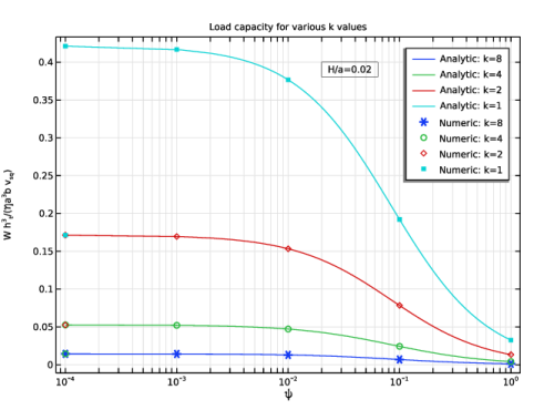
In the Settings window for 1D Plot Group, type Load Capacity for Various k Values in the Label text field.
3
Locate the Data section. From the Dataset list, choose None.
4
Locate the Title section. From the Title type list, choose Manual.
5
In the Title text area, type Load capacity for various k values.
6
Locate the Plot Settings section.
7
Select the x-axis label checkbox. In the associated text field, type \psi.
8
Select the y-axis label checkbox. In the associated text field, type W h<sup>3</sup><sub>t</sub>/(\eta a<sup>3</sup>b v<sub>sq</sub>).
9
Locate the Axis section. Select the x-axis log scale checkbox.
Function 1
1
In the Load Capacity for Various k Values toolbar, click  More Plots and choose Function.
2
In the Settings window for Function, locate the Data section.
3
From the Dataset list, choose Grid 1D 1.
4
Locate the y-Axis Data section. In the Expression text field, type 768*sum(sum(W_summand_psi(m, n, a, psi, 8, 0.02), n, 1, 15), m, 1, 15)/(pi^5).
5
Locate the x-Axis Data section. In the Expression text field, type psi.
6
In the Lower bound text field, type 1e-4.
7
Click to expand the Coloring and Style section. From the Color list, choose Cycle (reset).
8
Click to expand the Legends section. Select the Show legends checkbox.
9
From the Legends list, choose Manual.
10
Function 2
1
Right-click Function 1 and choose Duplicate.
2
In the Settings window for Function, locate the y-Axis Data section.
3
In the Expression text field, type 768*sum(sum(W_summand_psi(m, n, a, psi, 4, 0.02), n, 1, 15), m, 1, 15)/(pi^5).
4
Locate the Coloring and Style section. From the Color list, choose Cycle.
5
Locate the Legends section. In the table, enter the following settings:
Function 3
1
Right-click Function 2 and choose Duplicate.
2
In the Settings window for Function, locate the y-Axis Data section.
3
In the Expression text field, type 768*sum(sum(W_summand_psi(m, n, a, psi, 2, 0.02), n, 1, 15), m, 1, 15)/(pi^5).
4
Locate the Legends section. In the table, enter the following settings:
Function 4
1
Right-click Function 3 and choose Duplicate.
2
In the Settings window for Function, locate the y-Axis Data section.
3
In the Expression text field, type 768*sum(sum(W_summand_psi(m, n, a, psi, 1, 0.02), n, 1, 15), m, 1, 15)/(pi^5).
4
Locate the Legends section. In the table, enter the following settings:
Table Graph 1
1
In the Model Builder window, right-click Load Capacity for Various k Values and choose Table Graph.
2
In the Settings window for Table Graph, locate the Data section.
3
From the x-axis data list, choose psi.
4
From the Plot columns list, choose Manual.
5
In the Columns list box, select p*ht^3/(eta*a^3*b*sqvel).
6
Locate the Coloring and Style section. Find the Line style subsection. From the Line list, choose None.
7
From the Color list, choose Cycle (reset).
8
Find the Line markers subsection. From the Marker list, choose Cycle (reset).
9
Click to expand the Legends section. Select the Show legends checkbox.
10
From the Legends list, choose Manual.
11
Table Graph 2
1
Right-click Table Graph 1 and choose Duplicate.
2
In the Settings window for Table Graph, locate the Data section.
3
From the Table list, choose Table 2.
4
Locate the Coloring and Style section. From the Color list, choose Cycle.
5
Find the Line markers subsection. From the Marker list, choose Cycle.
6
Locate the Legends section. In the table, enter the following settings:
Table Graph 3
1
Right-click Table Graph 2 and choose Duplicate.
2
In the Settings window for Table Graph, locate the Data section.
3
From the Table list, choose Table 3.
4
Locate the Legends section. In the table, enter the following settings:
Table Graph 4
1
Right-click Table Graph 3 and choose Duplicate.
2
In the Settings window for Table Graph, locate the Data section.
3
From the Table list, choose Table 4.
4
Locate the Legends section. In the table, enter the following settings:
Annotation 1
1
In the Model Builder window, right-click Load Capacity for Various k Values and choose Annotation.
2
In the Settings window for Annotation, locate the Data section.
3
From the Dataset list, choose Study 1/Parametric Solutions 1 (sol2).
4
From the Parameter value (k,psi,Hbar) list, choose 1: k=8, psi=1, Hbar=0.02.
5
Locate the Annotation section. In the Text text field, type H/a=0.02.
6
Select the LaTeX markup checkbox.
7
Locate the Position section. In the X text field, type 0.02.
8
In the Y text field, type 0.4.
9
Locate the Advanced section. In the Precision text field, type 1.
10
Locate the Coloring and Style section. Clear the Show point checkbox.
11
Select the Show frame checkbox.
Load Capacity for Various k Values
1
In the Model Builder window, click Load Capacity for Various k Values.
2
In the Load Capacity for Various k Values toolbar, click  Plot.
Load Capacity for Various psi Values
1
In the Results toolbar, click  1D Plot Group.
2
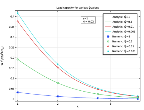
In the Settings window for 1D Plot Group, type Load Capacity for Various psi Values in the Label text field.
3
Locate the Data section. From the Dataset list, choose None.
4
Locate the Title section. From the Title type list, choose Manual.
5
In the Title text area, type Load capacity for various \psi values.
6
Locate the Plot Settings section.
7
Select the x-axis label checkbox. In the associated text field, type k.
8
Select the y-axis label checkbox. In the associated text field, type W h<sup>3</sup><sub>t</sub>/(\eta a<sup>3</sup>b v<sub>sq</sub>).
9
Locate the Axis section. Select the x-axis log scale checkbox.
Function 1
1
In the Load Capacity for Various psi Values toolbar, click  More Plots and choose Function.
2
In the Settings window for Function, locate the Data section.
3
From the Dataset list, choose Grid 1D 2.
4
Locate the y-Axis Data section. In the Expression text field, type 768*sum(sum(W_summand_psi(m, n, a, 1, k, 0.02), n, 1, 15), m, 1, 15)/(pi^5).
5
Locate the x-Axis Data section. In the Expression text field, type k.
6
In the Lower bound text field, type 1.
7
In the Upper bound text field, type 8.
8
Locate the Coloring and Style section. From the Color list, choose Cycle (reset).
9
Locate the Legends section. Select the Show legends checkbox.
10
From the Legends list, choose Manual.
11
Function 2
1
Right-click Function 1 and choose Duplicate.
2
In the Settings window for Function, locate the y-Axis Data section.
3
In the Expression text field, type 768*sum(sum(W_summand_psi(m, n, a, 0.1, k, 0.02), n, 1, 15), m, 1, 15)/(pi^5).
4
Locate the Coloring and Style section. From the Color list, choose Cycle.
5
Locate the Legends section. In the table, enter the following settings:
Function 3
1
Right-click Function 2 and choose Duplicate.
2
In the Settings window for Function, locate the y-Axis Data section.
3
In the Expression text field, type 768*sum(sum(W_summand_psi(m, n, a, 0.01, k, 0.02), n, 1, 15), m, 1, 15)/(pi^5).
4
Locate the Legends section. In the table, enter the following settings:
Function 4
1
Right-click Function 3 and choose Duplicate.
2
In the Settings window for Function, locate the y-Axis Data section.
3
In the Expression text field, type 768*sum(sum(W_summand_psi(m, n, a, 0.001, k, 0.02), n, 1, 15), m, 1, 15)/(pi^5).
4
Locate the Legends section. In the table, enter the following settings:
Table Graph 1
1
In the Model Builder window, right-click Load Capacity for Various psi Values and choose Table Graph.
2
In the Settings window for Table Graph, locate the Data section.
3
From the Table list, choose Table 5.
4
From the x-axis data list, choose k.
5
From the Plot columns list, choose Manual.
6
In the Columns list box, select p*ht^3/(eta*a^3*b*sqvel).
7
Locate the Coloring and Style section. Find the Line style subsection. From the Line list, choose None.
8
From the Color list, choose Cycle (reset).
9
Find the Line markers subsection. From the Marker list, choose Cycle (reset).
10
Locate the Legends section. Select the Show legends checkbox.
11
From the Legends list, choose Manual.
12
Table Graph 2
1
Right-click Table Graph 1 and choose Duplicate.
2
In the Settings window for Table Graph, locate the Data section.
3
From the Table list, choose Table 6.
4
Locate the Coloring and Style section. From the Color list, choose Cycle.
5
Find the Line markers subsection. From the Marker list, choose Cycle.
6
Locate the Legends section. In the table, enter the following settings:
Table Graph 3
1
Right-click Table Graph 2 and choose Duplicate.
2
In the Settings window for Table Graph, locate the Data section.
3
From the Table list, choose Table 7.
4
Locate the Legends section. In the table, enter the following settings:
Table Graph 4
1
Right-click Table Graph 3 and choose Duplicate.
2
In the Settings window for Table Graph, locate the Data section.
3
From the Table list, choose Table 8.
4
Locate the Legends section. In the table, enter the following settings:
Annotation 1
1
In the Model Builder window, right-click Load Capacity for Various psi Values and choose Annotation.
2
In the Settings window for Annotation, locate the Data section.
3
From the Dataset list, choose Mirror 3D 2.
4
From the Parameter value (k,psi,Hbar) list, choose 1: k=8, psi=1, Hbar=0.02.
5
Locate the Annotation section. In the Text text field, type a=1 \\ H = 0.02.
6
Select the LaTeX markup checkbox.
7
Locate the Position section. In the x text field, type 3.
8
In the y text field, type 0.4.
9
Locate the Coloring and Style section. Clear the Show point checkbox.
10
Select the Show frame checkbox.
Load Capacity for Various psi Values
1
In the Model Builder window, click Load Capacity for Various psi Values.
2
In the Load Capacity for Various psi Values toolbar, click  Plot.
Load Capacity for Various phi Values
1
In the Results toolbar, click  1D Plot Group.
2
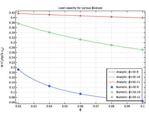
In the Settings window for 1D Plot Group, type Load Capacity for Various phi Values in the Label text field.
3
Locate the Data section. From the Dataset list, choose None.
4
Locate the Title section. From the Title type list, choose Manual.
5
In the Title text area, type Load capacity for various \phi values.
6
Locate the Plot Settings section.
7
Select the x-axis label checkbox. In the associated text field, type \phi.
8
Select the y-axis label checkbox. In the associated text field, type W h<sup>3</sup><sub>t</sub>/(\eta a<sup>3</sup>b v<sub>sq</sub>).
9
Locate the Legend section. From the Position list, choose Lower right.
Function 1
1
In the Load Capacity for Various phi Values toolbar, click  More Plots and choose Function.
2
In the Settings window for Function, locate the Data section.
3
From the Dataset list, choose Grid 1D 3.
4
Locate the y-Axis Data section. In the Expression text field, type 768*sum(sum(W_summand_phi(m, n, a, 5e-9, 1, H), n, 1, 15), m, 1, 15)/(pi^5).
5
Locate the x-Axis Data section. In the Expression text field, type H.
6
In the Lower bound text field, type 0.02.
7
In the Upper bound text field, type 0.1.
8
Locate the Coloring and Style section. From the Color list, choose Cycle (reset).
9
Locate the Legends section. Select the Show legends checkbox.
10
From the Legends list, choose Manual.
11
Function 2
1
Right-click Function 1 and choose Duplicate.
2
In the Settings window for Function, locate the y-Axis Data section.
3
In the Expression text field, type 768*sum(sum(W_summand_phi(m, n, a, 5e-10, 1, H), n, 1, 15), m, 1, 15)/(pi^5).
4
Locate the Coloring and Style section. From the Color list, choose Cycle.
5
Locate the Legends section. In the table, enter the following settings:
Function 3
1
Right-click Function 2 and choose Duplicate.
2
In the Settings window for Function, locate the y-Axis Data section.
3
In the Expression text field, type 768*sum(sum(W_summand_phi(m, n, a, 5e-11, 1, H), n, 1, 15), m, 1, 15)/(pi^5).
4
Locate the Legends section. In the table, enter the following settings:
Table Graph 1
1
In the Model Builder window, right-click Load Capacity for Various phi Values and choose Table Graph.
2
In the Settings window for Table Graph, locate the Data section.
3
From the Table list, choose Table 9.
4
From the x-axis data list, choose Hbar.
5
From the Plot columns list, choose Manual.
6
In the Columns list box, select p*ht^3/(eta*a^3*b*sqvel).
7
Locate the Coloring and Style section. Find the Line style subsection. From the Line list, choose None.
8
From the Color list, choose Cycle (reset).
9
Find the Line markers subsection. From the Marker list, choose Cycle (reset).
10
Locate the Legends section. Select the Show legends checkbox.
11
From the Legends list, choose Manual.
12
Table Graph 2
1
Right-click Table Graph 1 and choose Duplicate.
2
In the Settings window for Table Graph, locate the Data section.
3
From the Table list, choose Table 10.
4
Locate the Coloring and Style section. From the Color list, choose Cycle.
5
Find the Line markers subsection. From the Marker list, choose Cycle.
6
Locate the Legends section. In the table, enter the following settings:
Table Graph 3
1
Right-click Table Graph 2 and choose Duplicate.
2
In the Settings window for Table Graph, locate the Data section.
3
From the Table list, choose Table 11.
4
Locate the Legends section. In the table, enter the following settings:
Load Capacity for Various phi Values
1
In the Model Builder window, click Load Capacity for Various phi Values.
2
In the Load Capacity for Various phi Values toolbar, click  Plot.
Darcy Pressure and Velocity Fields
1
In the Results toolbar, click  3D Plot Group.
2
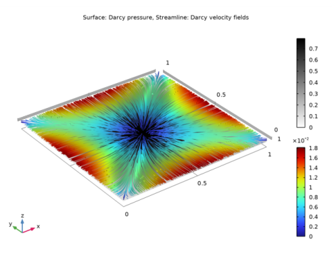
In the Settings window for 3D Plot Group, type Darcy Pressure and Velocity Fields in the Label text field.
3
Locate the Data section. From the Dataset list, choose Mirror 3D 2.
4
From the Parameter value (k,psi,Hbar) list, choose 18: k=1, psi=0.01, Hbar=0.02.
5
Click to expand the Selection section. Click to expand the Title section. From the Title type list, choose Manual.
6
In the Title text area, type Surface: Darcy pressure, Streamline: Darcy velocity fields.
7
Locate the Plot Settings section. Clear the Plot dataset edges checkbox.
8
Locate the Color Legend section. From the Position list, choose Right double.
Surface 1
1
Right-click Darcy Pressure and Velocity Fields and choose Surface.
2
In the Settings window for Surface, locate the Expression section.
3
In the Expression text field, type p*ht^3/(eta*a^2*sqvel).
4
Locate the Coloring and Style section. From the Color table list, choose GrayScale.
5
From the Color table transformation list, choose Reverse.
Selection 1
1
Right-click Surface 1 and choose Selection.
2
In the Settings window for Selection, locate the Selection section.
3
From the Selection list, choose Thin-Film Boundary.
Streamline 1
1
In the Model Builder window, right-click Darcy Pressure and Velocity Fields and choose Streamline.
2
In the Settings window for Streamline, locate the Expression section.
3
In the x-component text field, type dl.u*dl.rho*a/eta.
4
In the y-component text field, type dl.v*dl.rho*a/eta.
5
In the z-component text field, type dl.w*dl.rho*a/eta.
6
Locate the Streamline Positioning section. From the Positioning list, choose Starting-point controlled.
7
In the Points text field, type 2000.
8
Locate the Coloring and Style section. Find the Point style subsection. From the Type list, choose Arrow.
Color Expression 1
1
Right-click Streamline 1 and choose Color Expression.
2
In the Settings window for Color Expression, locate the Expression section.
3
In the Expression text field, type dl.U*dl.rho*a/eta.
Darcy Pressure and Velocity Fields
1
In the Model Builder window, under Results click Darcy Pressure and Velocity Fields.
2
In the Darcy Pressure and Velocity Fields toolbar, click  Plot.
3
Click the  Zoom Extents button in the Graphics toolbar.