|
|
|

|
1
|
|
2
|
|
1
|
|
2
|
|
3
|
Click in the Graphics window and then press Ctrl+A to select all domains.
|
|
4
|
|
5
|
|
6
|
|
7
|
|
1
|
|
2
|
|
3
|
Select the Design Module Boolean operations checkbox.
|
|
4
|
|
5
|
Browse to the model’s Application Libraries folder and double-click the file sports_car_fsi_geom_sequence.mph.
|
|
6
|
|
7
|
Click OK.
|
|
1
|
In the Model Builder window, expand the Component 1 (comp1) > Geometry 1 > Mirror node, then click Fillet 11 (fil11).
|
|
2
|
|
1
|
|
2
|
|
3
|
|
4
|
|
5
|
Clear the Automatic detection of small details checkbox.
|
|
1
|
|
2
|
Go to the Add Material window.
|
|
3
|
|
4
|
Click the Add to Component button in the window toolbar.
|
|
5
|
|
6
|
Click the Add to Component button in the window toolbar.
|
|
7
|
|
1
|
|
2
|
|
1
|
|
2
|
|
3
|
Clear the Automatic detection of small details checkbox.
|
|
4
|
|
1
|
|
2
|
Go to the Add Physics window.
|
|
3
|
|
4
|
Find the Physics interfaces in study subsection. In the table, clear the Solve checkboxes for Study 1, Study 2, and Study 3.
|
|
5
|
Click the Add to Component 2 button in the window toolbar.
|
|
6
|
|
1
|
|
2
|
Click
|
|
3
|
|
4
|
|
5
|
|
6
|
In the Dependent variable quantity table, enter the following settings:
|
|
7
|
In the Source term quantity table, enter the following settings:
|
|
8
|
|
9
|
|
10
|
|
11
|
In the Dependent variables (Pa) table, enter the following settings:
|
|
1
|
In the Model Builder window, under Component 2 (comp2) > Weak Form Boundary PDE (wb) click Weak Form PDE 1.
|
|
2
|
|
3
|
In the weak text-field array, type test(Tstress1)*(Tstress1-comp1.genext1(comp1.spf.T_tracx)) on the first row.
|
|
4
|
In the weak text-field array, type test(Tstress2)*(Tstress2-comp1.genext1(comp1.spf.T_tracy)) on the second row.
|
|
5
|
In the weak text-field array, type test(Tstress3)*(Tstress3-comp1.genext1(comp1.spf.T_tracz)) on the third row.
|
|
1
|
|
2
|
Go to the Add Study window.
|
|
3
|
Find the Physics interfaces in study subsection. In the table, clear the Solve checkboxes for LES RBVM (spf), Incompressible Potential Flow (ipf), and Turbulent Flow, k-ε 2 (spf2).
|
|
4
|
|
5
|
Click the Add Study button in the window toolbar.
|
|
6
|
|
1
|
|
2
|
|
3
|
Click to expand the Values of Dependent Variables section. Find the Values of variables not solved for subsection. From the Settings list, choose User controlled.
|
|
4
|
|
5
|
|
6
|
|
7
|
In the Time (s) list, choose 0.6 s (2), 0.602 s, 0.604 s, 0.606 s, 0.608 s, 0.61 s, 0.612 s, 0.614 s, 0.616 s, 0.618 s, 0.62 s, 0.622 s, 0.624 s, 0.626 s, 0.628 s, 0.63 s, 0.632 s, 0.634 s, 0.636 s, 0.638 s, 0.64 s, 0.642 s, 0.644 s, 0.646 s, 0.648 s, 0.65 s, 0.652 s, 0.654 s, 0.656 s, 0.658 s, 0.66 s, 0.662 s, 0.664 s, 0.666 s, 0.668 s, 0.67 s, 0.672 s, 0.674 s, 0.676 s, 0.678 s, 0.68 s, 0.682 s, 0.684 s, 0.686 s, 0.688 s, 0.69 s, 0.692 s, 0.694 s, 0.696 s, 0.698 s, and 0.7 s.
|
|
8
|
Click to expand the Store in Output section. In the table, enter the following settings:
|
|
1
|
|
2
|
|
3
|
|
4
|
|
5
|
|
6
|
Click to expand the Mesh Selection section. In the table, enter the following settings:
|
|
7
|
Click to expand the Store in Output section. In the table, enter the following settings:
|
|
1
|
|
2
|
|
3
|
|
4
|
|
5
|
|
6
|
|
7
|
In the Model Builder window, expand the Study 4 > Solver Configurations > Solution 4 (sol4) > Time-Dependent Solver 1 node, then click Fully Coupled 1.
|
|
8
|
|
9
|
|
10
|
|
1
|
|
2
|
|
3
|
|
4
|
|
1
|
|
2
|
|
3
|
|
4
|
|
1
|
|
2
|
|
1
|
|
2
|
|
3
|
From the list, choose User-controlled mesh.
|
|
1
|
|
2
|
|
3
|
|
4
|
|
1
|
|
2
|
|
3
|
|
4
|
Click
|
|
1
|
|
2
|
|
3
|
|
1
|
|
2
|
In the Settings window for Global, click Add Expression in the upper-right corner of the y-Axis Data section. From the menu, choose Component 2 (comp2) > Definitions > Variables > F_mirror - Norm of mirror force - N.
|
|
3
|
Click Add Expression in the upper-right corner of the y-Axis Data section. From the menu, choose Component 2 (comp2) > Definitions > Variables > F_window - Norm of window force - N.
|
|
4
|
|
1
|
|
2
|
|
3
|
|
4
|
In the Parameter values (freq (Hz)) list, choose 10, 20, 30, 40, 50, 60, 70, 80, 90, 100, 110, 120, 130, 140, 150, 160, 170, 180, 190, 200, 210, 220, 230, 240, 250, 260, 270, 280, 290, 300, 310, 320, 330, 340, 350, 360, 370, 380, 390, 400, 410, 420, 430, 440, 450, 460, 470, 480, 490, 500, 510, 520, 530, 540, 550, 560, 570, 580, 590, 600, 610, 620, 630, 640, 650, 660, 670, 680, 690, 700, 710, 720, 730, 740, 750, 760, 770, 780, 790, 800, 810, 820, 830, 840, 850, 860, 870, 880, 890, 900, 910, 920, 930, 940, 950, 960, 970, 980, 990, 1000, 1010, 1020, 1030, 1040, 1050, 1060, 1070, 1080, 1090, 1100, 1110, 1120, 1130, 1140, 1150, 1160, 1170, 1180, 1190, 1200, 1210, 1220, 1230, 1240, 1250, 1260, 1270, 1280, 1290, 1300, 1310, 1320, 1330, 1340, 1350, 1360, 1370, 1380, and 1390.
|
|
5
|
Locate the Plot Settings section.
|
|
6
|
|
7
|
|
8
|
|
9
|
|
1
|
|
2
|
|
1
|
|
2
|
|
1
|
|
2
|
|
1
|
|
2
|
|
3
|
|
4
|
|
1
|
|
2
|
Go to the Add Physics window.
|
|
3
|
|
4
|
Find the Physics interfaces in study subsection. In the table, clear the Solve checkboxes for Study 1, Study 2, Study 3, and Study 4.
|
|
5
|
Click the Add to Component 2 button in the window toolbar.
|
|
6
|
|
1
|
|
2
|
|
1
|
|
2
|
|
3
|
|
4
|
|
1
|
In the Model Builder window, under Component 2 (comp2) > Shell (shell) click Thickness and Offset 1.
|
|
2
|
|
3
|
|
1
|
|
2
|
|
3
|
|
4
|
|
1
|
|
2
|
|
3
|
|
4
|
|
1
|
|
2
|
|
3
|
|
4
|
|
1
|
|
2
|
|
3
|
|
1
|
|
2
|
|
3
|
|
4
|
|
1
|
|
3
|
|
4
|
|
1
|
|
2
|
|
3
|
|
4
|
|
5
|
|
1
|
|
2
|
Go to the Add Study window.
|
|
3
|
Find the Physics interfaces in study subsection. In the table, clear the Solve checkboxes for LES RBVM (spf), Incompressible Potential Flow (ipf), Turbulent Flow, k-ε 2 (spf2), and Weak Form Boundary PDE (wb).
|
|
4
|
Find the Studies subsection. In the Select Study tree, select Preset Studies for Selected Physics Interfaces > Frequency Domain, Modal.
|
|
5
|
Click the Add Study button in the window toolbar.
|
|
6
|
|
1
|
|
2
|
|
3
|
Locate the Physics and Variables Selection section. Select the Modify model configuration for study step checkbox.
|
|
4
|
|
5
|
Right-click and choose Disable.
|
|
6
|
Click to expand the Store in Output section. In the table, enter the following settings:
|
|
1
|
|
2
|
|
3
|
|
4
|
Click to expand the Mesh Selection section. In the table, enter the following settings:
|
|
5
|
Click to expand the Store in Output section. In the table, enter the following settings:
|
|
1
|
|
2
|
|
1
|
|
2
|
|
4
|
|
1
|
|
2
|
|
3
|
|
4
|
|
1
|
|
2
|
Go to the Result Templates window.
|
|
3
|
|
4
|
Click the Add Result Template button in the window toolbar.
|
|
5
|
|
1
|
|
2
|
|
3
|
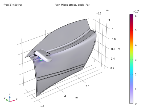
Locate the Plot Settings section. From the View list, choose New view to create a dedicated view for this plot that you can adjust independently.
|
|
4
|
|
1
|
|
2
|
Go to the Result Templates window.
|
|
3
|
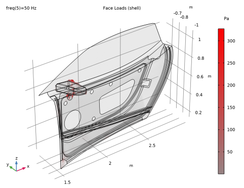
In the tree, select Study 5/Solution 6 (9) (sol6) > Shell > Applied Loads (shell) > Face Loads (shell).
|
|
4
|
Click the Add Result Template button in the window toolbar.
|
|
5
|
|
1
|
|
2
|
|
3
|
|
4
|